The Laplacian in RL
Hey nerds! Today I’ll be implementing another paper on the graph Laplacian applied to RL, “The Laplacian in RL: Learning Representations with Efficient Approximations” (2018), by Wu, Tucker, and Nachum.
It’s a very cool paper and I learned a lot going through it and coding it up. I view it as the next in a progression from some other papers I did posts on before, Mahadevan’s proto value function (PVF) paper (2005), and Machado et al’s eigenoptions paper (2017).
I’m really gonna try this time to just center the post around the results, and keep the yapping to a minimum. So check out those and my previous Laplacian posts for more background!
A little background and motivation
In this paper, they want to find the eigenfunctions of the (graph) Laplacian. The motivation is the same as elsewhere: the eigenfunctions capture some inherent structure of the environment, so let’s take it as a given that they’re useful for all sorts of things in RL.
The two earlier papers I mentioned above did this, but in much simpler ways. The PVF paper assumes you can just construct the Laplacian matrix and do eigendecomposition. The eigenoptions paper instead builds a matrix from sampled transitions, calculates the SVD of that matrix, and shows that the eigenvectors from the SVD can be good approximations to the eigenfunctions of the Laplacian.
Both cool! But you might notice a distinct lack of our universal hammer, neural networks. The methods above basically do some linear algebra to get the eigenfunctions we want, but we’d like to be able to use the power and flexibility of NNs, which is what this paper adds.
A teensy bit of math and the main idea
For states $S$, an eigenfunction is a function $f: S \rightarrow \mathbb R$ that satisfies the eigenvalue equation $L f_k = \lambda_k f_k$. We usually want several eigenfunctions, so if we want $d$ of them, we’re really looking for a function $\phi(s) = [f_1(s), \dots, f_d(s)] \in \mathbb R^d$. This is what we want the NN to learn.
To do this, their clever insight is that you can use the Graph Drawing objective (GDO), from the Koren paper I did a post on here. The main idea is that in addition to the eigenfunctions being the solutions to the eigenvalue equation, they’re also the functions that minimize the quadratic form:
\[E(f_k) = f_k^\intercal L f_k = \sum_{i, j} w_{ij} (f_k^{(i)} - f_k^{(j)})^2\]such that they’re all orthonormal to each other, $f_k^\intercal f_l = \delta_{kl}$.
This viewpoint offers a different objective we can use to find the eigenfunctions! To find them using this GDO, we need to make a differentiable objective for the NN that includes both of these parts, the GDO/quadratic form itself, and the orthonormality constraint.
However, in the original graph drawing paper, it’s assumed that 1) there are a finite/reasonable number of graph nodes, and 2) we just know the edge weights $w_{ij}$. In this paper, neither of those are true: 1) the method must work for continuous/large state spaces, and 2) the edge weights are related to the state-transition probabilities, which are generally unknown in RL. So, some modifications have to be made.
To make a long story short (check out the paper for the full story!) both of these problems are basically solved by sampling. The GDO can be written as an expectation over the stationary distribution $\rho$ and env transitions $P^\pi$:
\[G(f_1, \dots, f_d) = \mathbb E_{u \sim \rho, v \sim P^\pi (v \mid u)} \bigg[ \sum_{k}^d (f_k(u) - f_k(v))^2 \bigg]\]and the constraint violation can be expressed as a penalty, which can be written as an expectation over pairs of independent samples from the stationary distribution:
\[\mathbb E_{u \sim \rho, v \sim \rho} \bigg[ \sum_{j, k}^d (f_j(u) f_k(u) - \delta_{jk}) (f_j(v) f_k(v) - \delta_{jk}) \bigg]\]As is typical, the constraint violation just gets added to the primary objective as a penalty with a magic coefficient $\beta$ :
\[\tilde G(f_1, \dots, f_d) = G(f_1, \dots, f_d) + \beta \mathbb E_{u \sim \rho, v \sim \rho} \bigg[ \sum_{j, k}^d (f_j(u) f_k(u) - \delta_{jk}) (f_j(v) f_k(v) - \delta_{jk}) \bigg]\]Since both terms are expectations, they can be approximated with samples from those distributions.
From a high level, that’s most of what’s going on!
Experiments
Alllrighty, let’s try and implement a few of the things they show in the paper, and a few extras.
Gap to optimal, comparison with Machado et al’s eigenoptions
In section 5.1, they show the results of some experiments with a toy maze env that has a small number of states, which allows them to do some analysis that we can’t do for the more general case that this method is designed for. They compare their method to two previous ones from Machado et al, but I’ll only be comparing it to the “transition” one (red curve) below.
Here’s their figure, which I’ll be trying to make:
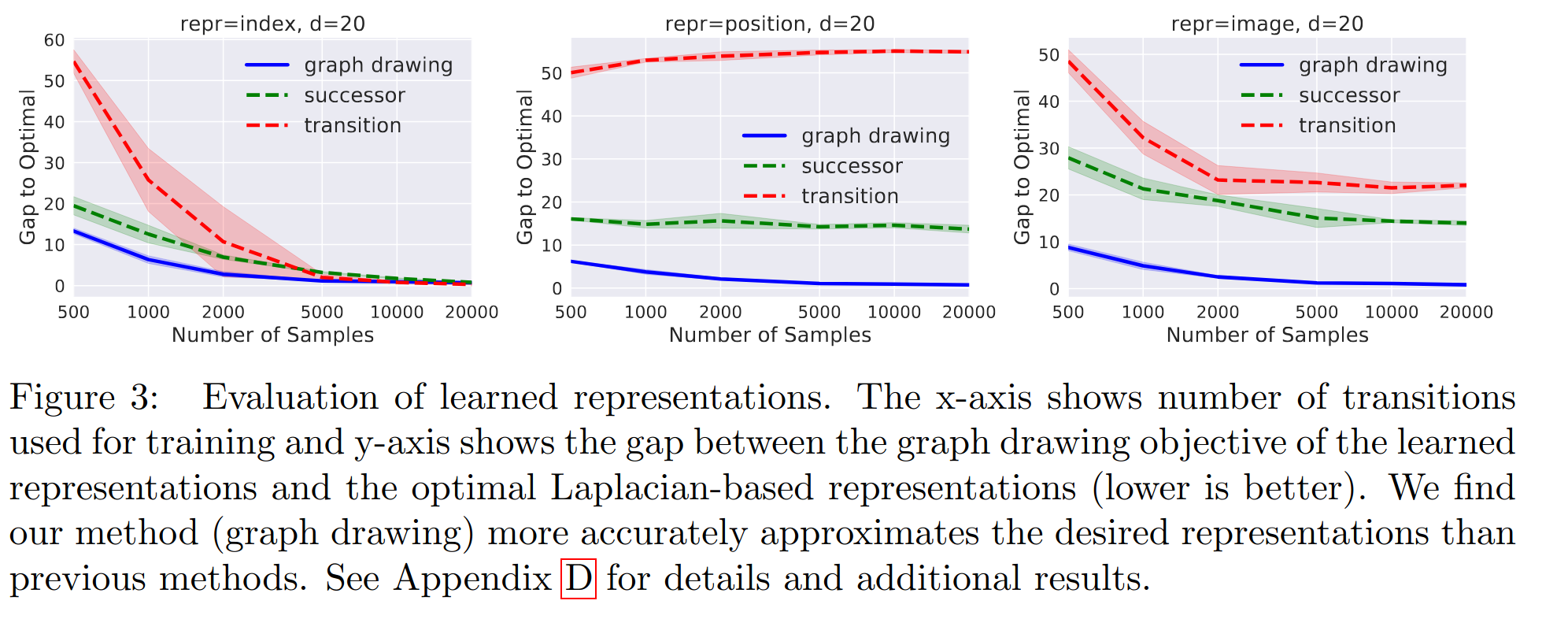
The idea is to use each method (theirs and previous ones) to learn a representation with a limited number of transition samples, and see how each method’s performance improves as that number of samples increases.
The env is this little 4-rooms maze:
![]()
which is a $15 \times 15$ grid, with $152$ non-wall states (the white cells). The actions are just movement in the four cardinal directions, going against a wall results in a no-op, etc.
They try each method with three different state representations (SR) $\psi(s) \in \mathbb R^m$ (since that’s another benefit of their method), namely:
1) a one-hot vector (length $152$ in this case) where the agent’s cell index is 1, 2) a coordinates representation that’s the agent’s $(x, y)$ coordinates you see in the maze above, normalized to be in $[-1, 1]^2$, and 3) an image based one that’s a $15 \times 15 \times 3$ RGB image, where the agent’s cell is colored red
So, for a given method, state representation, embedding dimension $d$, and number of transitions $N$, here’s the process:
- sample $N$ transitions from the environment
- learn the representation $\phi(s) = [f_1(s), \dots, f_d(s)] \in \mathbb R^d$
- embed all states with the learned $\phi$, and calculate the $d$ principal directions of them using SVD
- call these principal directions a new representation $\phi’$, and embed all transitions with $\phi’$
- see how this $\phi’$ does on the GDO, compared to the optimal of the true eigenfunctions (the “gap to optimal” on the y-axis)
Here’s what I get:
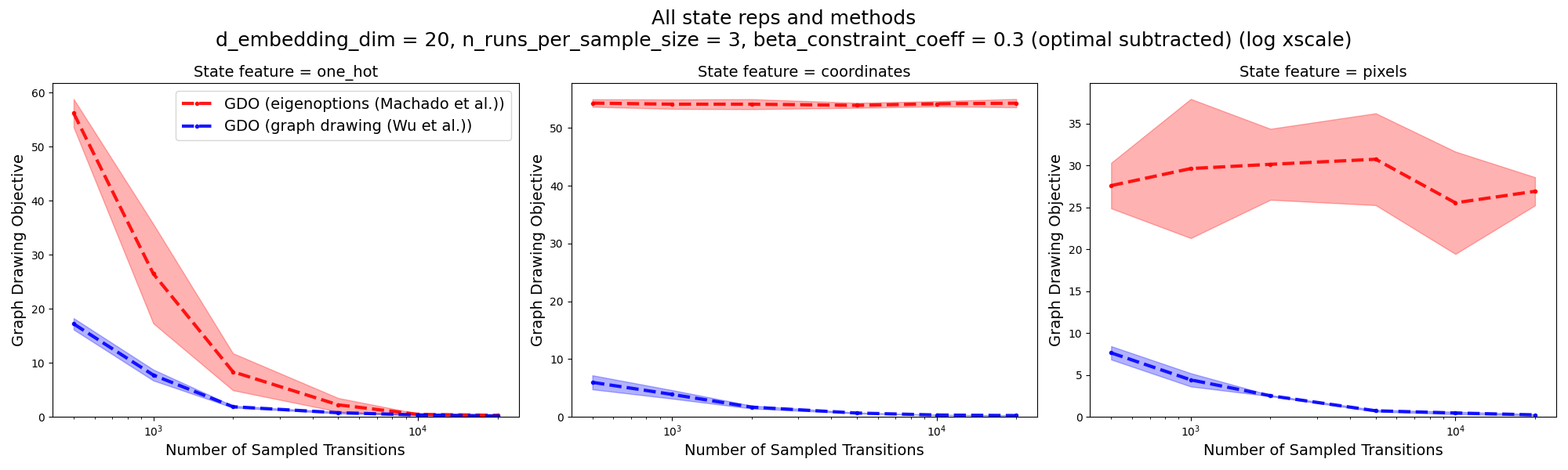
Not bad! It has ballpark the right numbers, and definitely the right shapes. Note that (like theirs above), the x-axis has a log scale. The takeaways we’re supposed to get from this are that 1) their method beats the eigenoptions method at almost all numbers of samples, and 2) for most state representations, and 3) the gap to optimal goes to zero with enough samples for their method, but only goes to zero for one-hot SR for the eigenoptions method.
That said… there’s actually a lot going on here that I’m now pretty unsure about. I’ll leave that for the end. Let’s keep it moving and go to the next part.
Beta ablation
Recall that $\beta$ is the Lagrange multiplier for the orthonormality constraint penalty:
\[\tilde G(f_1, \dots, f_d) = G(f_1, \dots, f_d) + \beta \mathbb E_{u \sim \rho, v \sim \rho} \bigg[ \sum_{j, k} (f_j(u) f_k(u) - \delta_{jk}) (f_j(v) f_k(v) - \delta_{jk}) \bigg]\]They add that constraint penalty term to turn it into an unconstrained problem, but what $\beta$ should we use? The “true” problem is $\beta = \infty$ (i.e., a hard constraint), but we have to use some $\beta < \infty$ to turn it into an unconstrained optimization problem. We’d like to use as large a $\beta$ as possible, but larger $\beta$ makes the optimization problem harder in practice.
So they do an ablation over $\beta$ values, and have this figure:
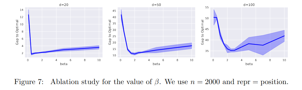
which I’ll be trying to reproduce. This is important, since I suspect there might be enough slight differences between my implementation and theirs that the good $\beta$ values they found wouldn’t work as well for me, so I want to find good $\beta$ values for my setup, that I’ll use for the other experiments (I actually used the values found here for the “gap to optimal” ones above).
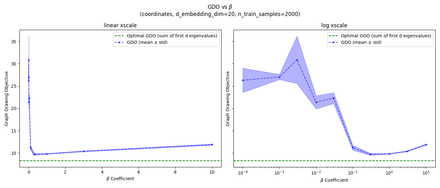
I’m just gonna be doing it for $d=20$, since that’s what’s in the main gap to optimal figure, and the others don’t seem very different anyway. But I will be doing it for all three SRs. I’ll also do it for both 2k and 20k samples, because 2k is what they use in Figure 7 above, but 20k is the “full” dataset size, so I’d like to have the best $\beta$ for it (for other experiments below).
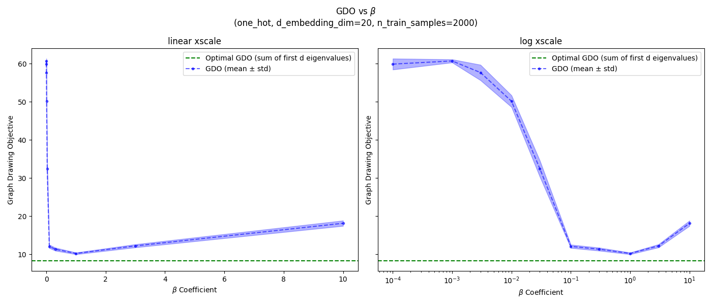
Here’s what I got for 2k samples:
![]()
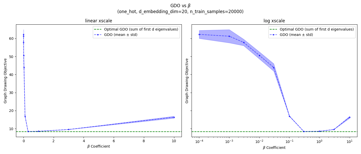
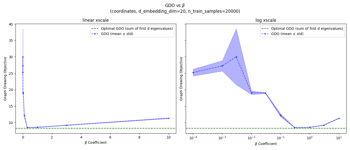
and 20k samples:
![]()
Hey hey, not bad. Note that I put a linear x scale plot on the left, and log x scale on the right. It looks like for 2k samples, the best values are:
- one-hot: ${1.0}$
- coordinates: ${0.3, 1.0}$
- pixels: ${0.3, 1.0, 3.0}$
and for 20k samples:
- one-hot: ${0.3, 1.0, 3.0}$
- coordinates: ${0.3, 1.0, 3.0}$
- pixels: ${0.3, 1.0, 3.0}$
It seems like $\beta = 1.0$ is a good value for all SRs and dataset sizes, so I’ll use that.
One more thing: the GDO in those plots increases with larger $\beta$, since it’s a harder optimization problem. But you might notice that it also increases with very small $\beta$, which might seem weird because small $\beta$ means that it could minimize the GDO without having to worry about satisfying the constraint as much. What gives?
I think this is due to their evaluation procedure above. After learning $\phi$, they embed all states with it and use SVD to find the $d$ principal directions, and those are what they actually use to calculate the GDO. So for a small $\beta$, the naive $\phi$ values we find probably would have a small GDO, but of course they don’t satisfy the orthogonality constraint. So once they’re converted to their principal directions (which do satisfy the orthogonality constraint), they’re now much worse for the GDO.
Reward shaping
Pushing on! At the beginning, we said to assume that the eigenfunctions of the Laplacian are definitely useful. Here’s one example of how they can be.
If we want to do general goal conditioned RL (check out my previous posts on GCRL), we want a general goal-conditioned reward that our agent can use. A standard one is a negative distance from the current state to the goal state, $r(s, g) = -\Vert s - g \Vert$, but it has pitfalls I talked about in this post.
Most notably, it depends a lot on the specific state representation and norm used. As a good example, they have this figure in the paper:
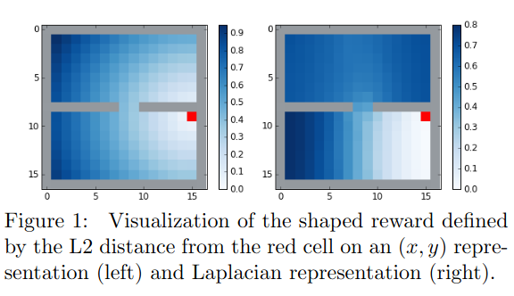
Basically, one solution is to find an embedding for states, $\phi(s)$, and then define the reward as a (negative) distance in that space: $r(s, g) = -\Vert \phi(s) - \phi(g) \Vert$. And wouldn’t ya know it, we happen to have just the embedding you might be interested in!
So, yeah, that’s pretty much it. You define the GCRL reward function based on a learned embedding as above, and then use it to do GCRL.
They have this image of this reward function for three different mazes, which I’ll be trying to make:
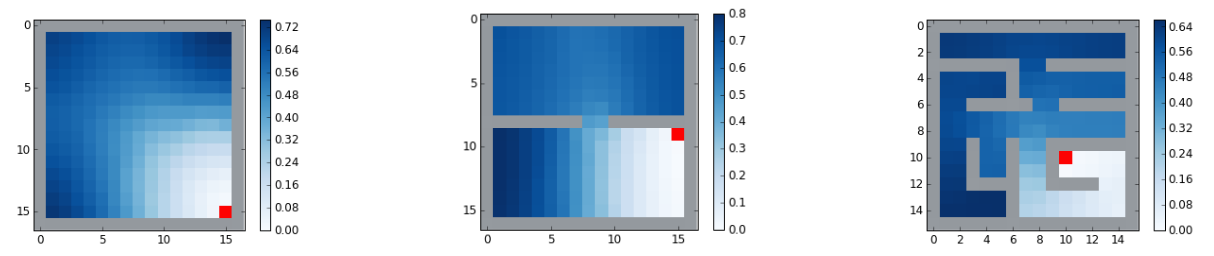
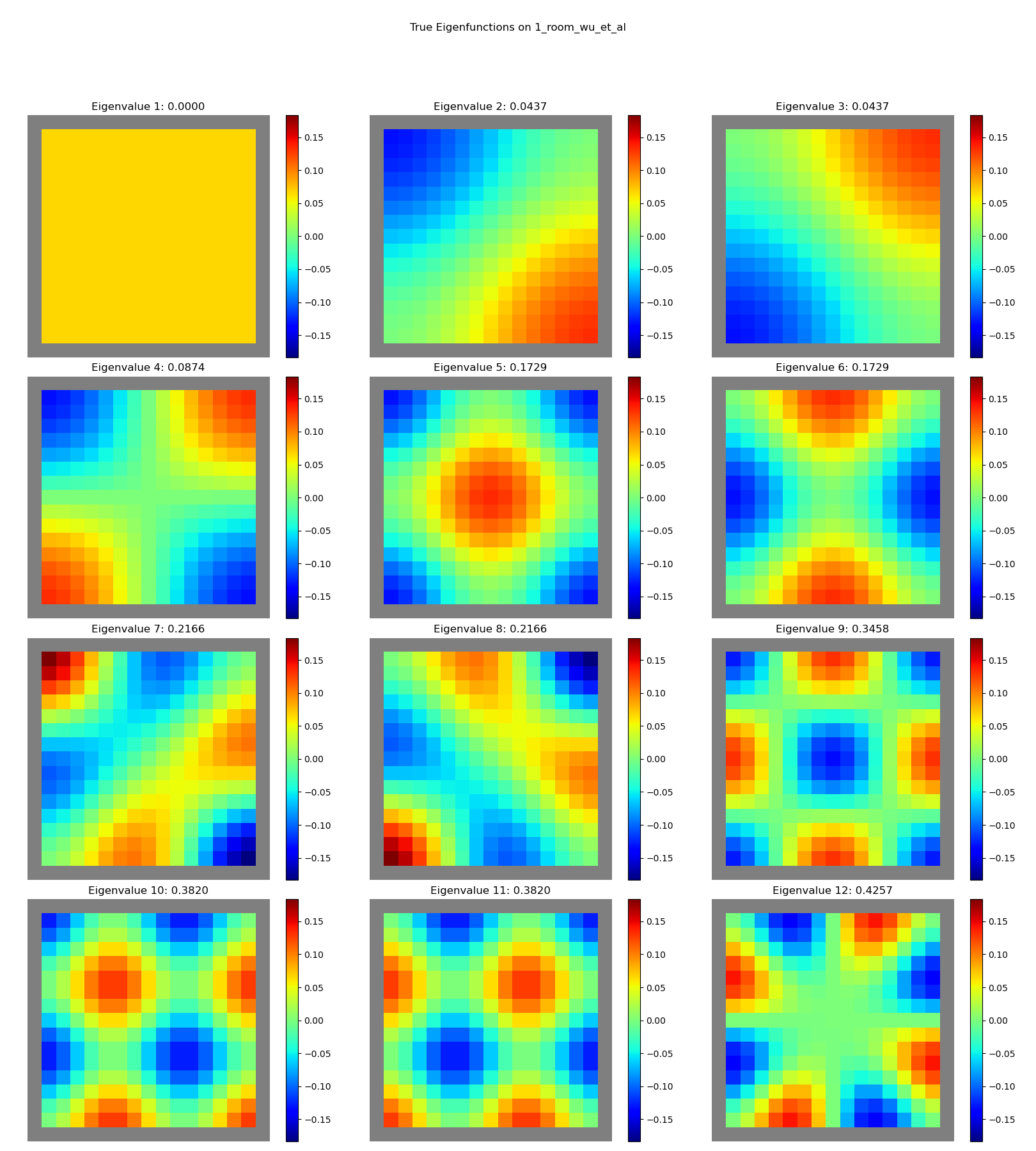
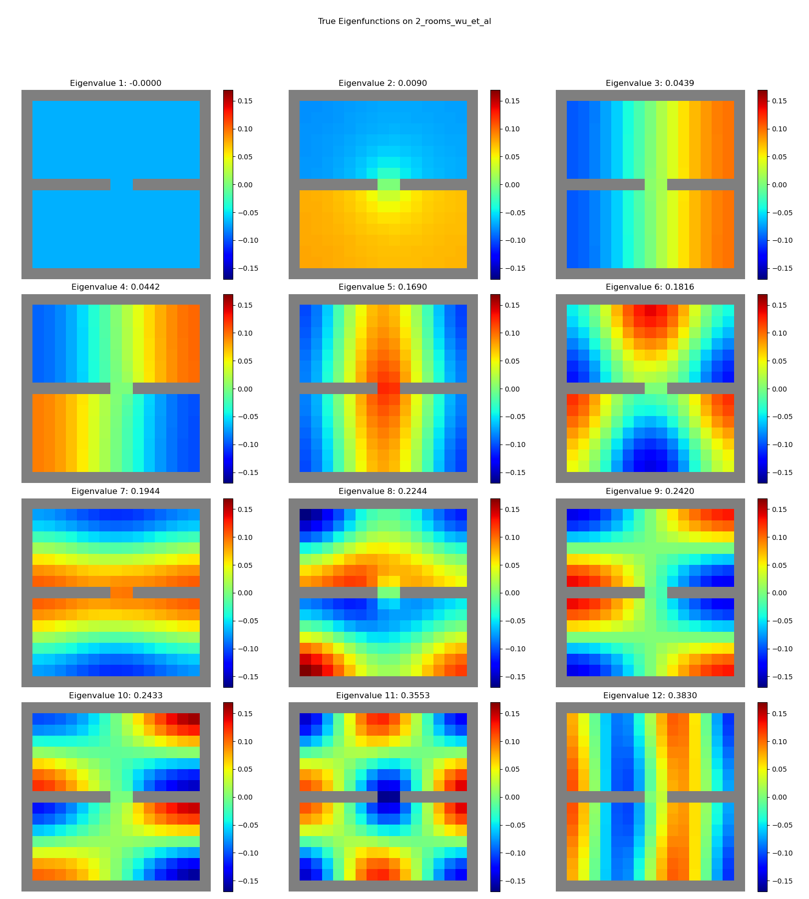
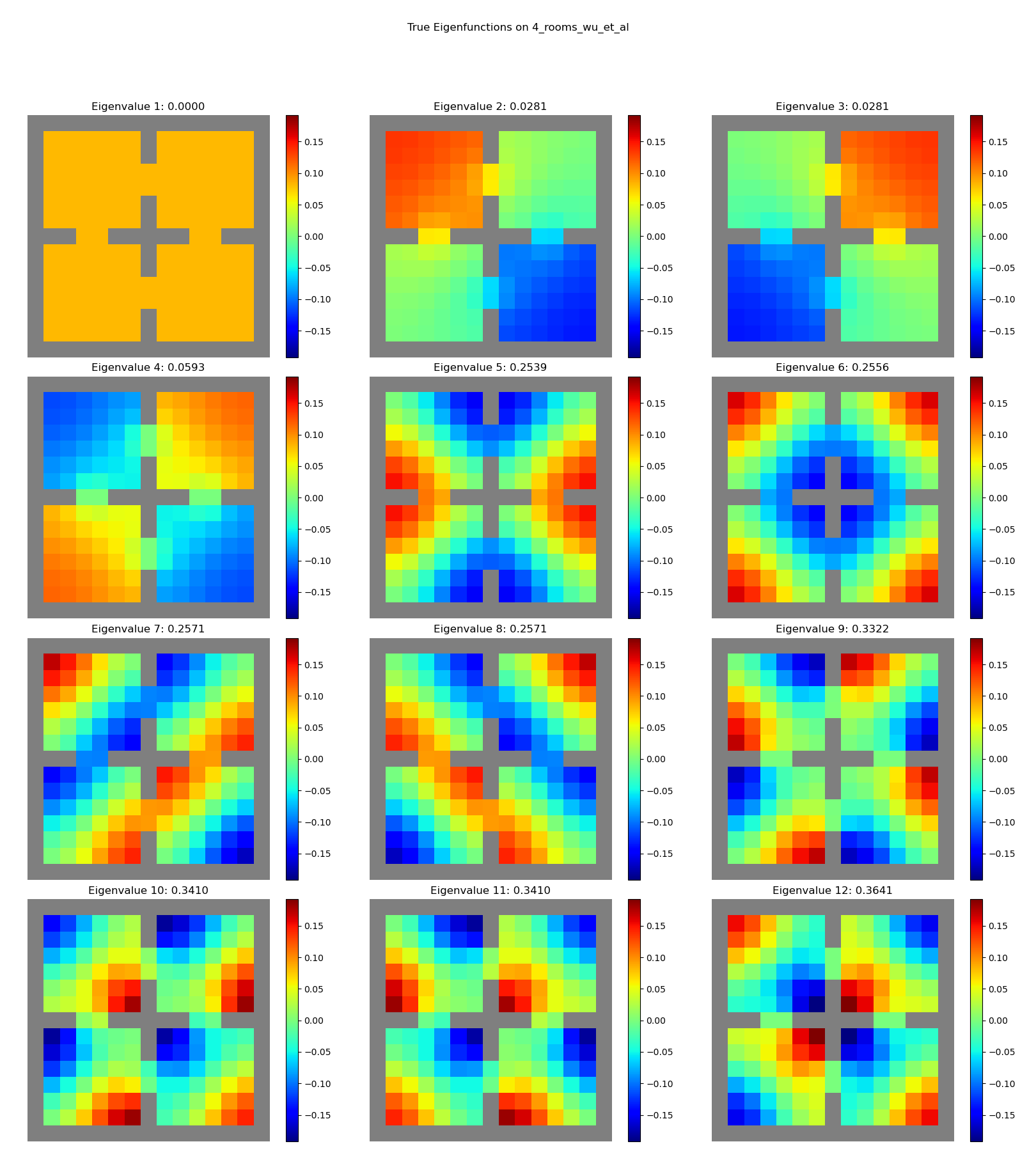
First, let’s actually make these with the true eigenfunctions (which we can just solve for) as a sanity check. So to be clear, I’m finding the eigenfunctions of each maze using np.linalg.eigh on the Laplacian matrix defined by the adjacency matrix.
In the appendix, they say they use $d = 20$ for the gridworld reward shaping experiments. So if I use the first 20 true eigenfunctions for the mazes above, I get:
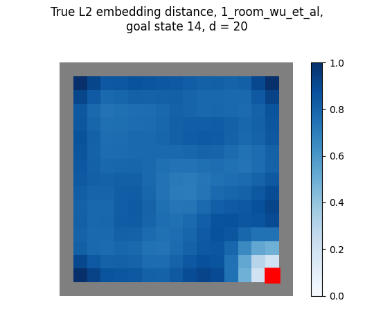
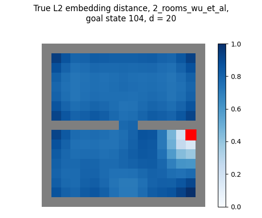
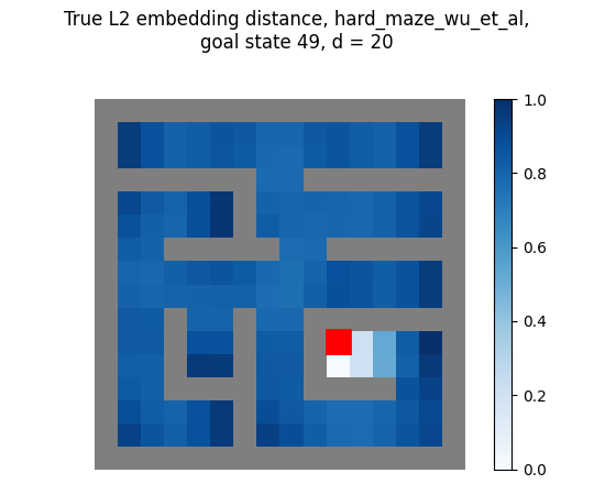
huh! Those look different than theirs… Let’s look at the same thing, but for all the $d$ values up to 20:
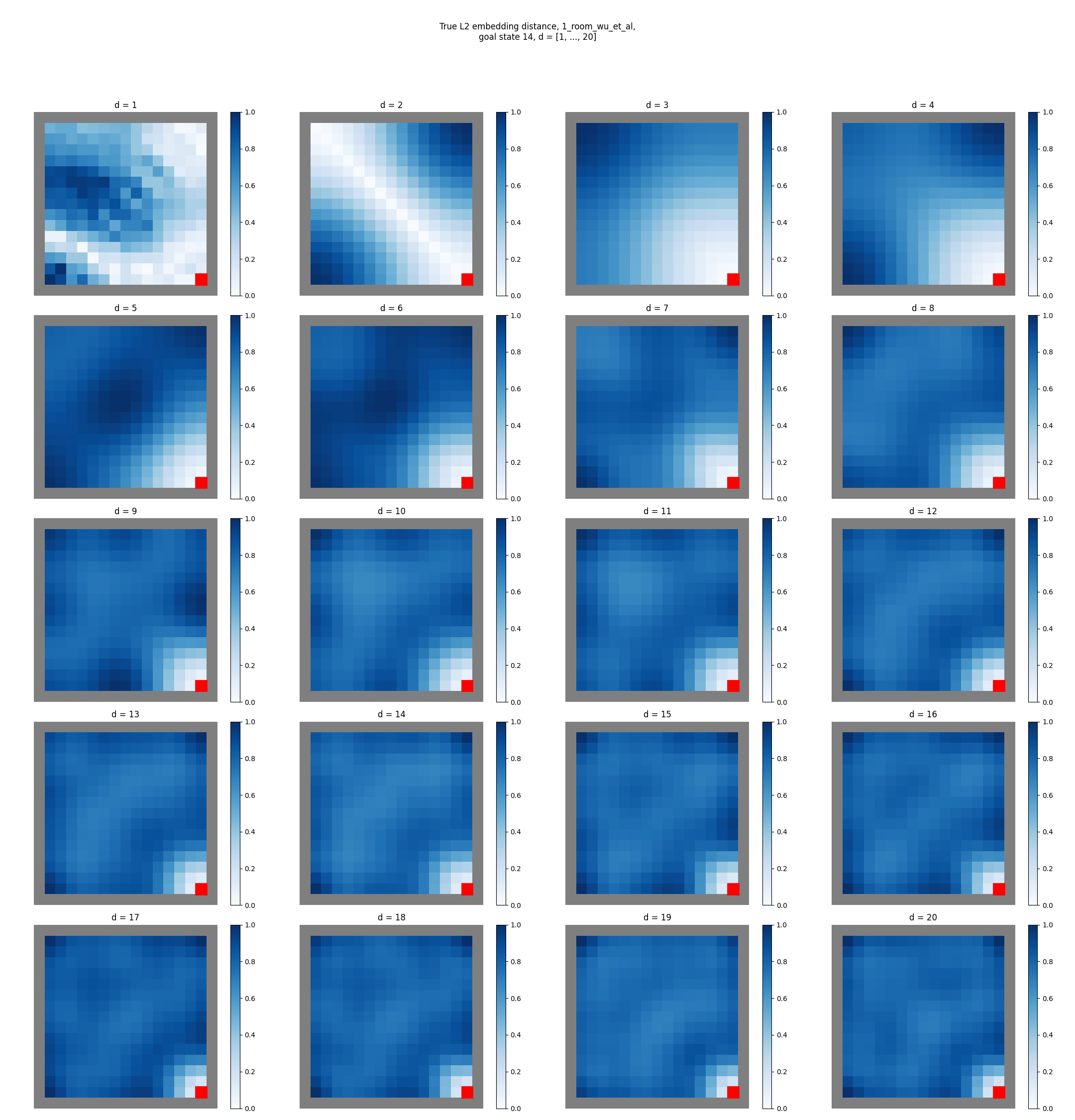
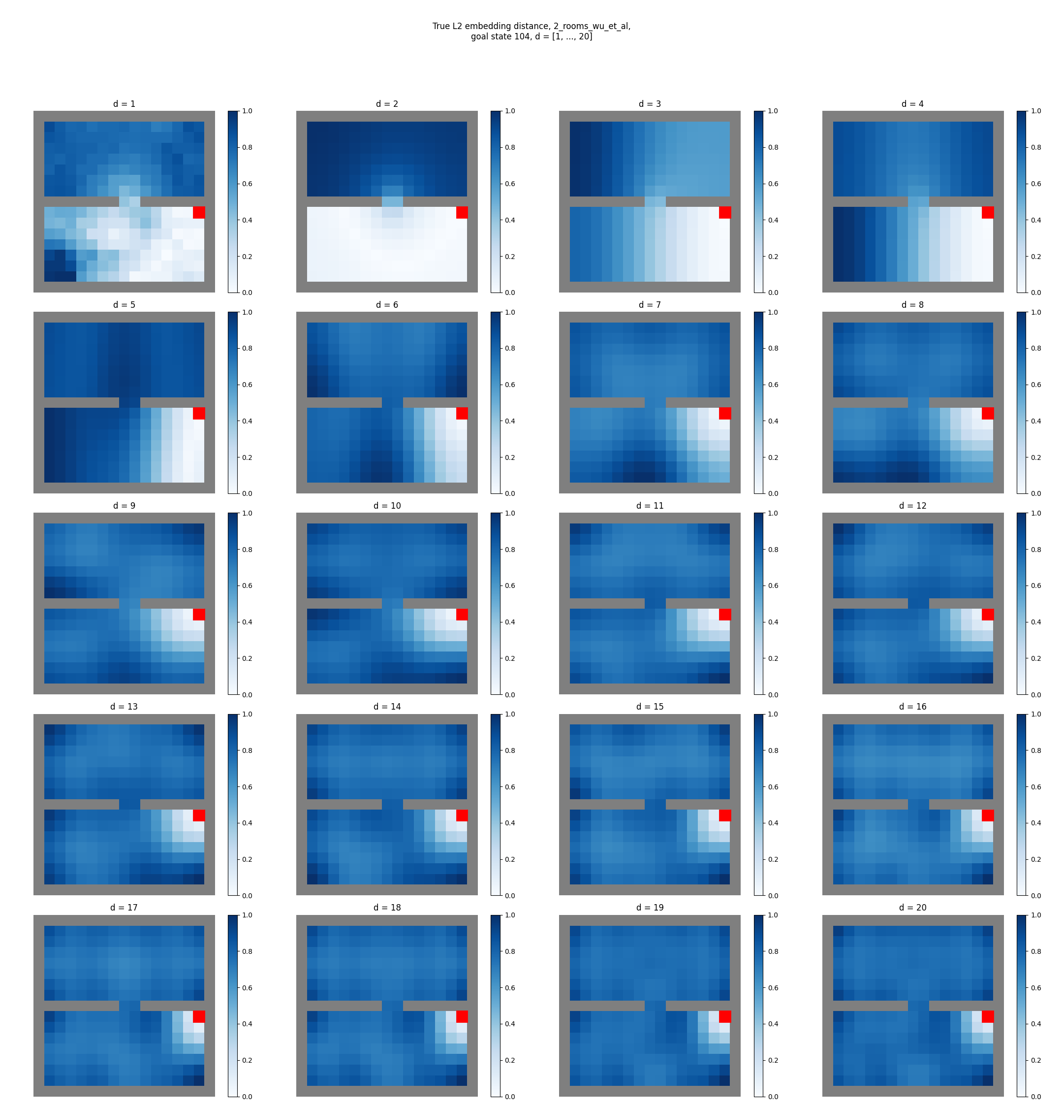
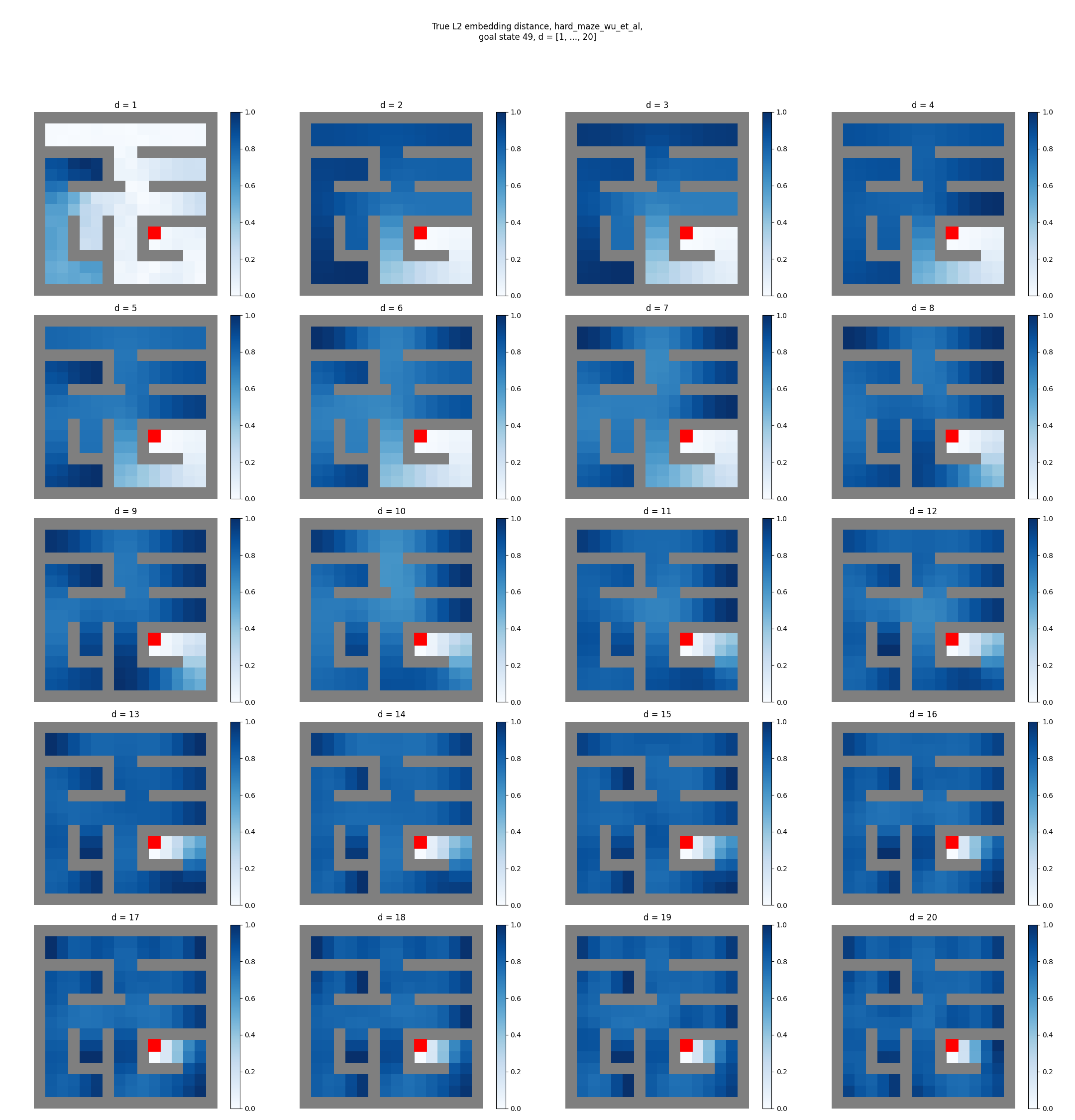
You can see that for each, as we increase $d$, it seems like it has the effect of “washing out” the reward function at most distances away from the goal (note that the $d=1$ embedding distance looks a bit weird, because it contains only 1st eigenfunction which is ~constant, but I divide each embedding distance by its max, which magnifies those very small differences).
And, to get the shaping reward that looks most similar to theirs, we have to use a much smaller $d$:
- for the 1 room maze, $d = 3$ or $d=4$ look closest
- for the 2 room maze, $d = 4$ looks closest
- for the hard maze, $d = 3$ looks closest
That said, these are the true eigenfunctions, and therefore probably of better quality in some way. Now let’s try it with the learned embeddings. There are a few details here I won’t go into too deeply, but a few big differences they do from the earlier stuff are:
- They use $\delta_{jj} = 0.05$ in the constraint (rather than $1$)
- The transitions they use for training here aren’t just typical one-step, i.e., $(s_i, s_{i+1})$ transitions – they sample multi-step transitions, i.e., $(s_i, s_{i+k})$
- They use $\beta = 5$, which is larger than the minimum that both they and I find for the $\beta$ ablation (but maybe is counteracting the $\delta$ value above?)
My true eigenfunctions above weren’t calculated with those first two differences (the $\beta$ one isn’t relevant for it), and they do effectively change the graph structure, so I wouldn’t be surprised if that could cause a difference.
Anyway, I ran it with those changes, which gives this:
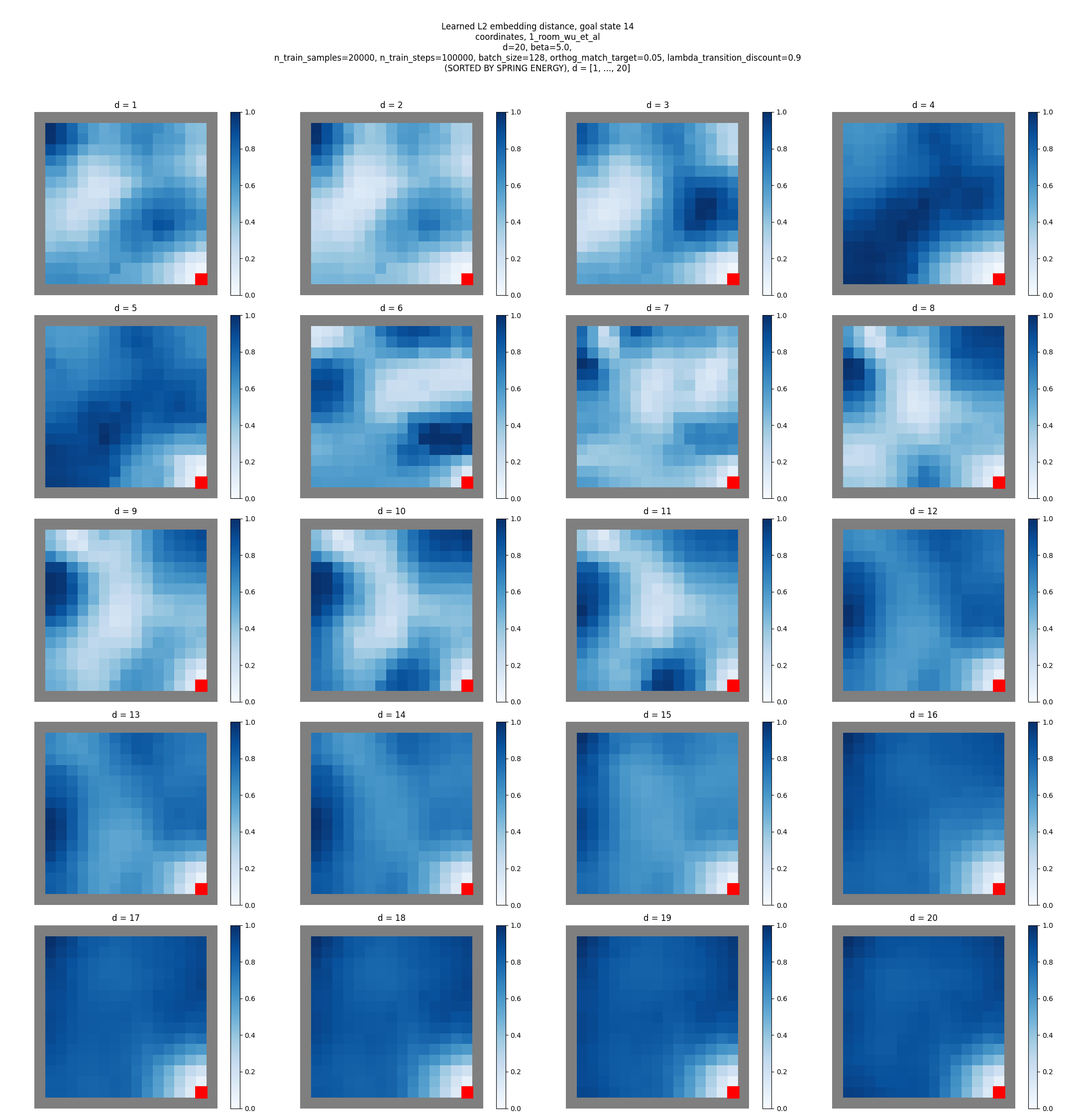
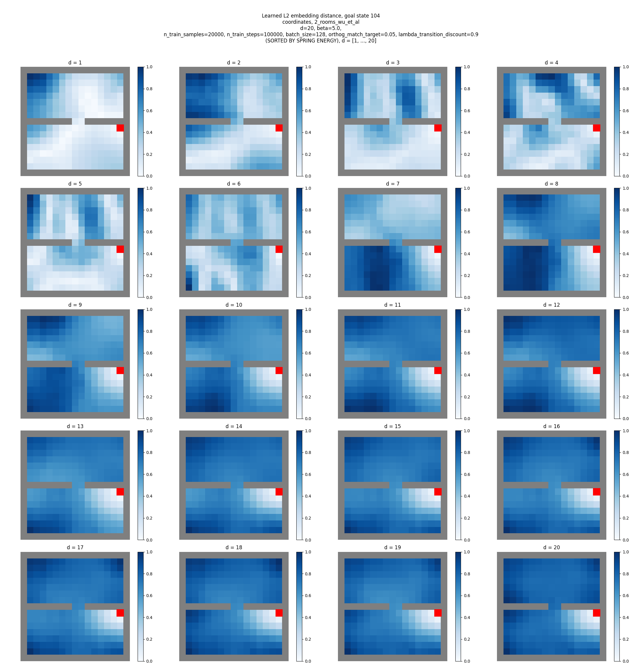
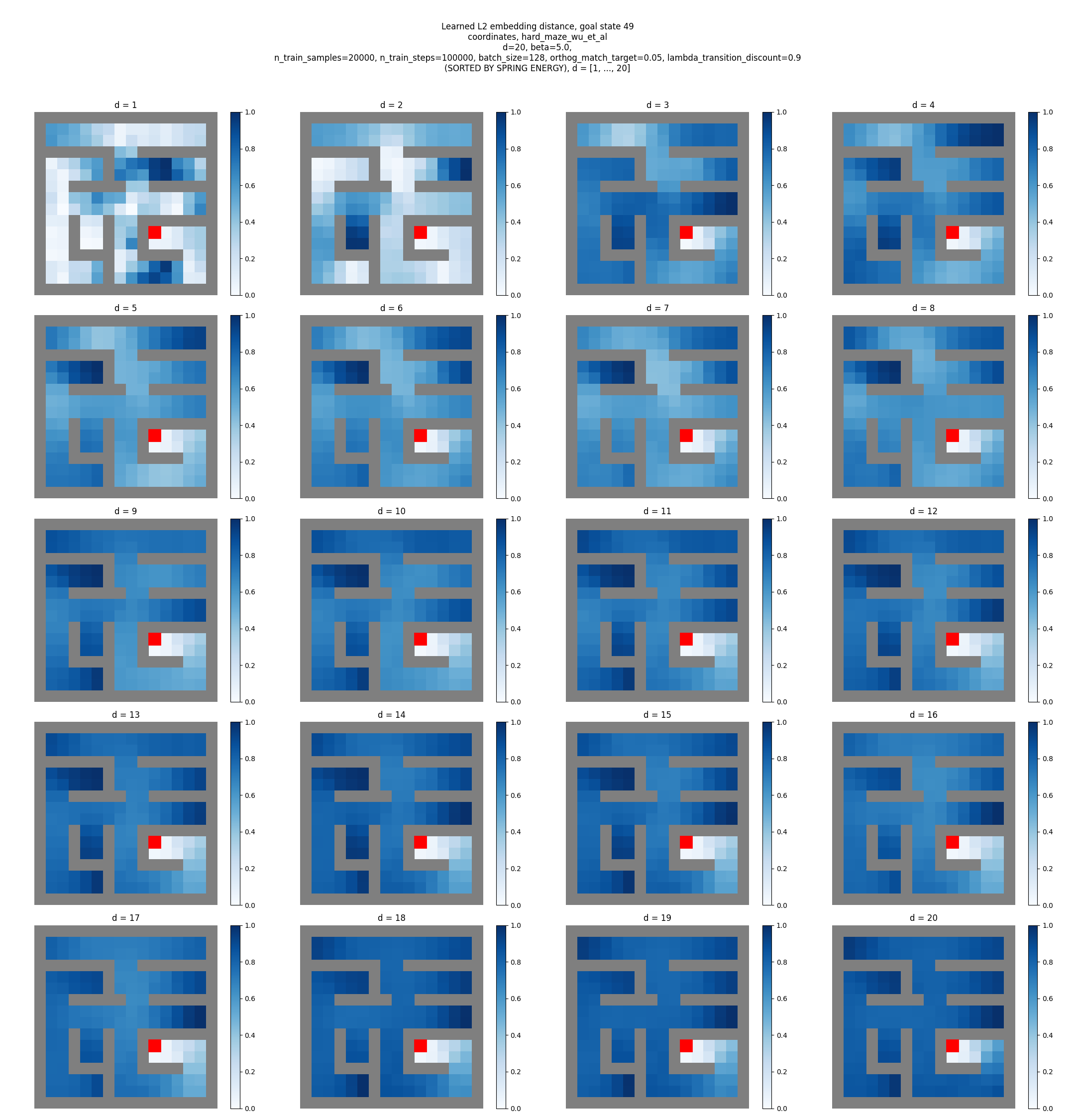
For reference again, here are theirs:
Hmmm. So mine clearly still clearly don’t look like theirs for $d = 20$, or really any $d$ for that matter. Maybe it’s just a scaling issue, but it seems like the light colored region close to the goal extends a lot further in theirs, whereas it gets quickly washed out to near the average for mine.
They also do a whole thing with mixing the reward derived from this with a regular L2 distance reward (i.e., the L2 distance not in the embedding space), but I’ll talk about that later.
Visualizing embeddings
Let’s also look at the actual embeddings learned by the models. They didn’t do this in the paper, but it’s always interesting (and besides, I need a fun thumbnail for the post :P ).
There are a few variants for us to look at:
- for the true eigenfunctions vs the paper’s method
- for the different state representations
- for the different mazes
I’m only gonna do the one-hot and coordinates SRs, since I think the pixels one is kinda redundant (see discussion at end).
True eigenfunctions
Let’s first look at the true ones, for comparison. There’s no state representation here, since we’re just using the underlying graph.
1 room:
2 rooms:
4 rooms:
hard maze:
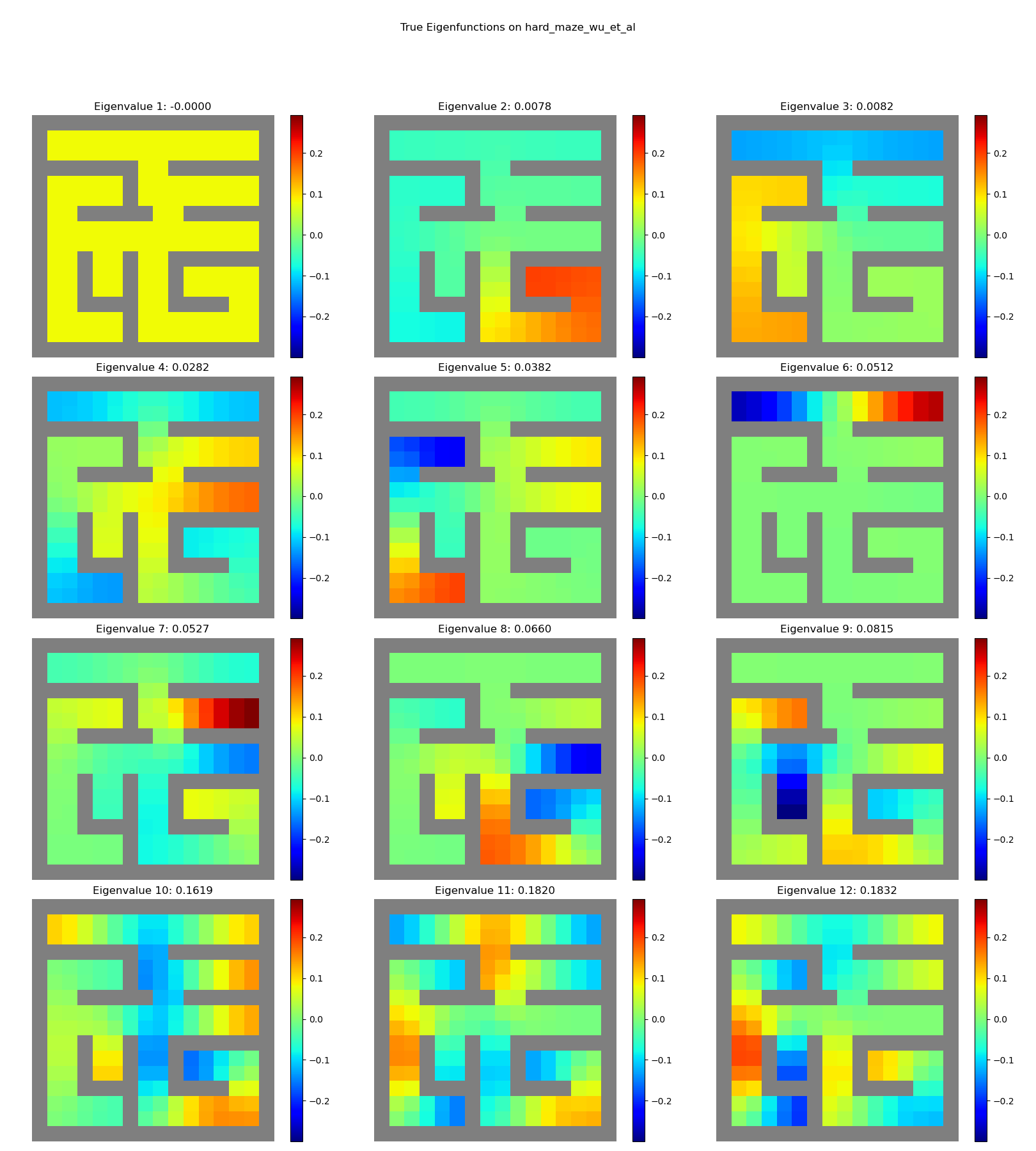
Sweeeeeet. You can see clear structure, with “vibrational modes” and all.
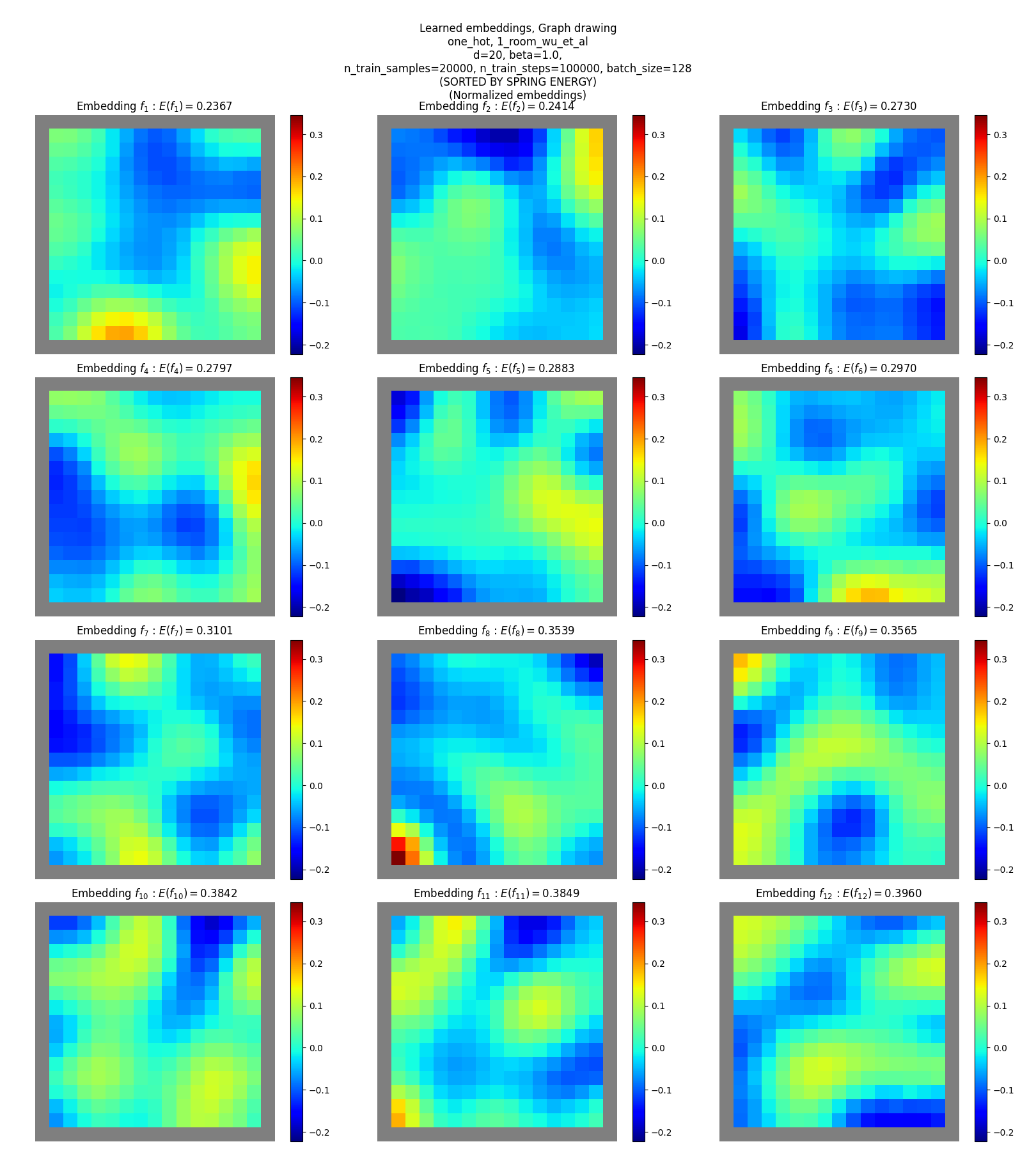
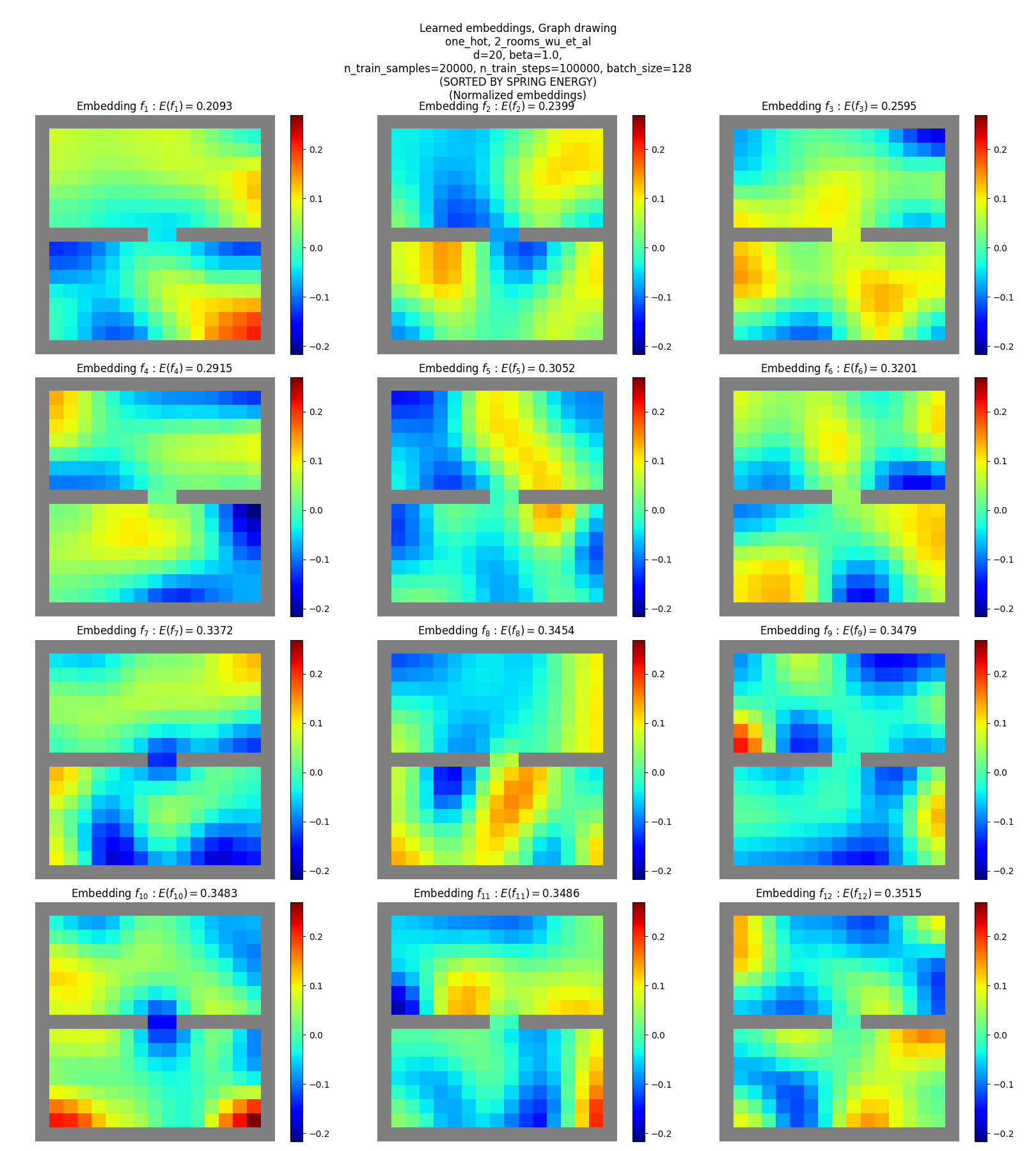
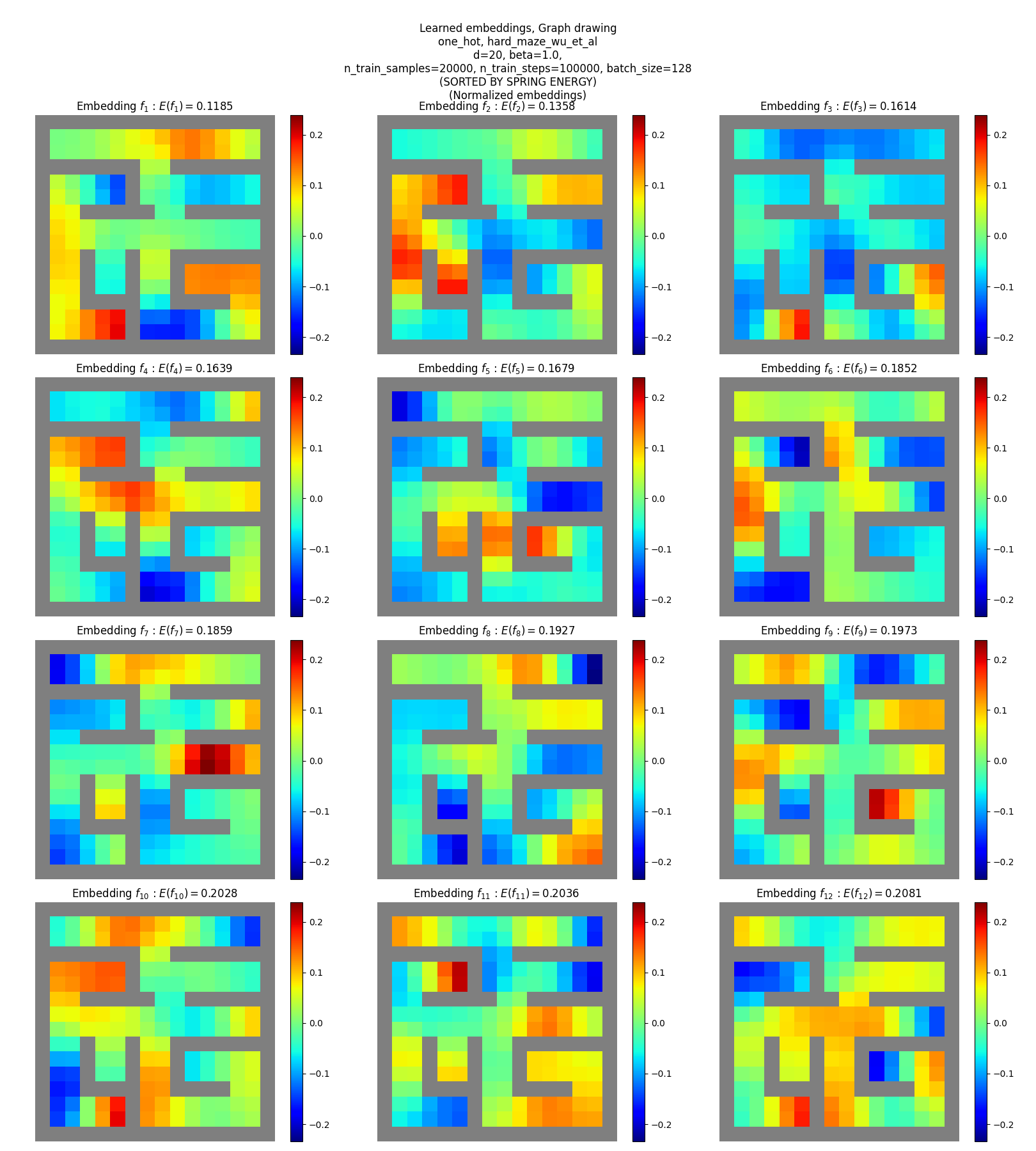
Graph drawing embeddings
One-hot SR
Coordinates SR
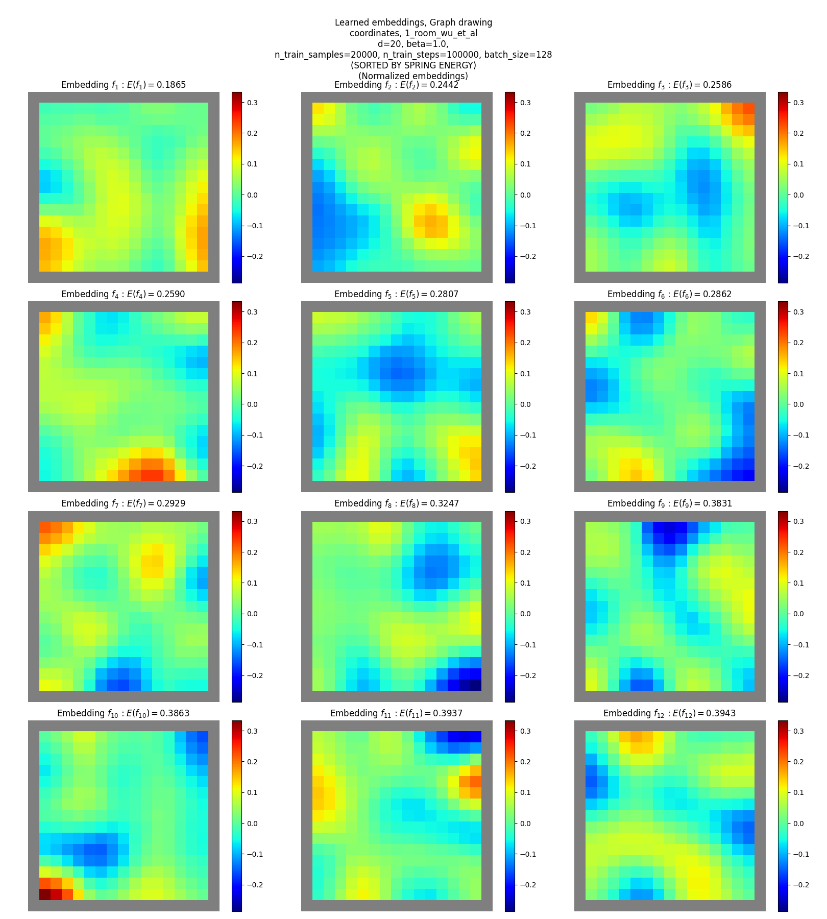
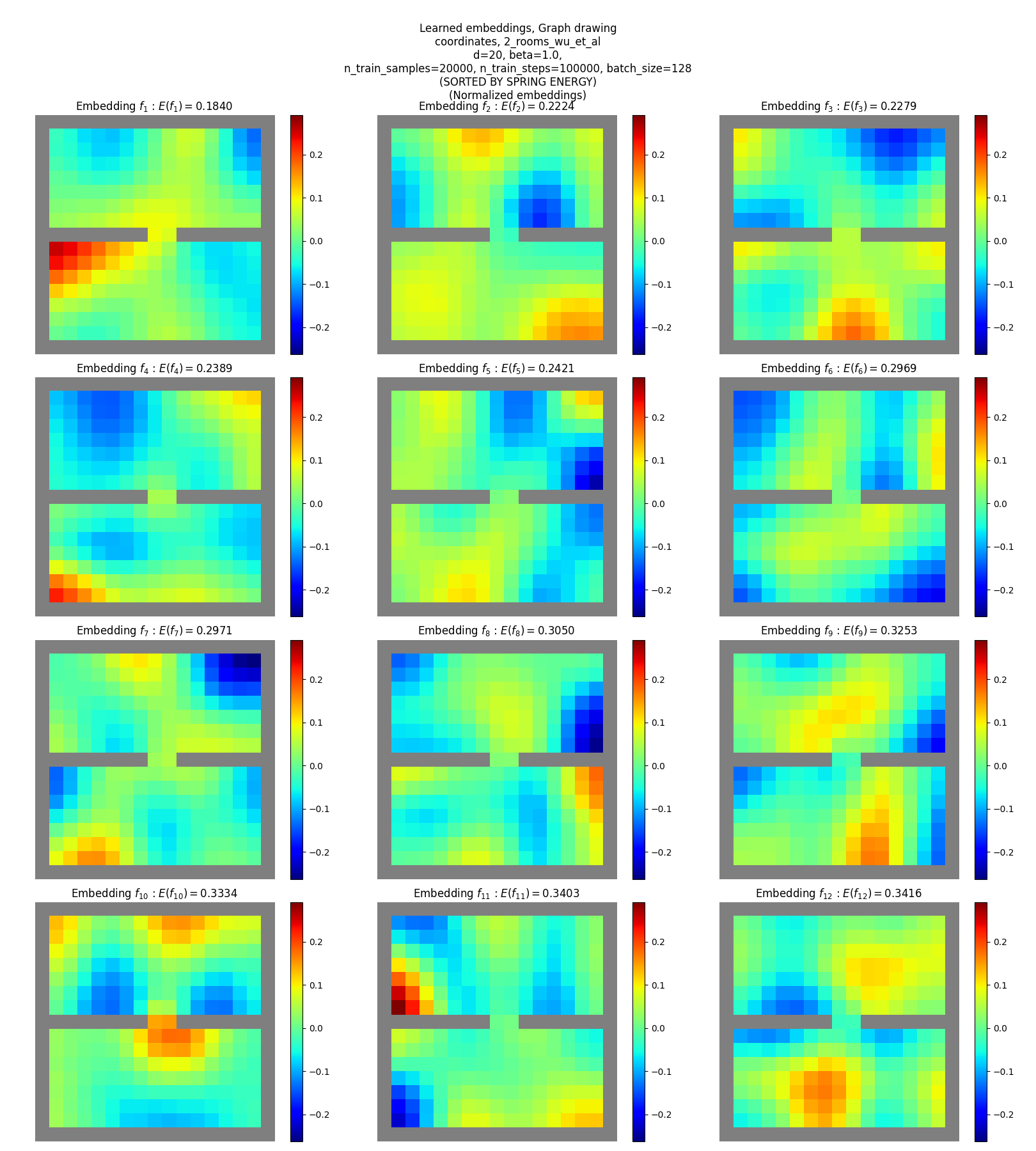
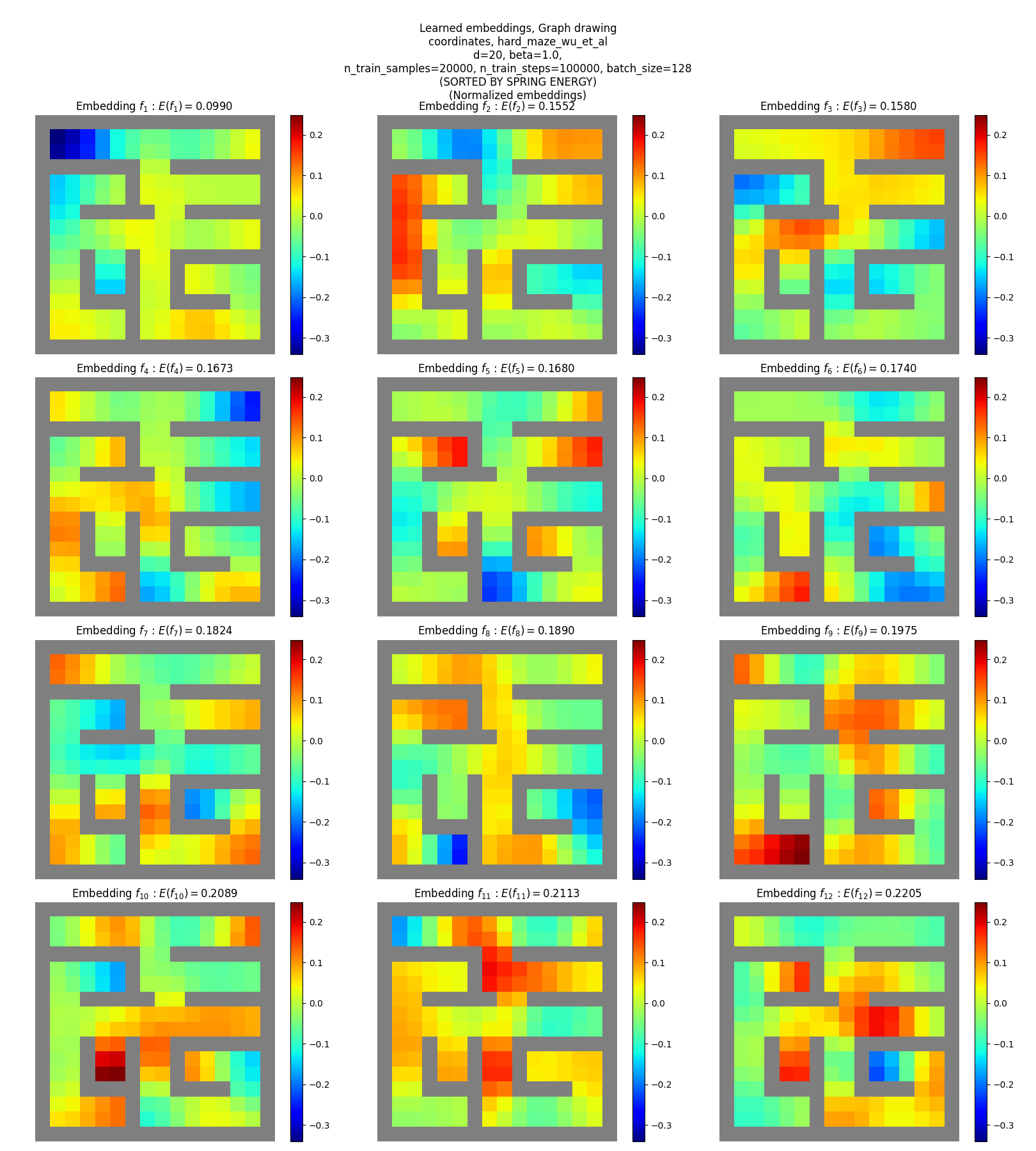
You can see that:
- they don’t match the true eigenfunctions at all, except plausibly slightly for the hard maze
- they don’t have as clear “patterns” or “structure”, except for maybe a little in terms of around some corners and edges (but could just be reading into noise)
Yet, these are reasonable solutions for the objective. How? Read on!
Embedding energies
Lastly, let’s look at the per-eigenfunction energies found for the different methods. Recall that the “energy” of a function $f$ is $\langle f, L f \rangle$, and the energy of an eigenfunction $f_j$ is its eigenvalue $\lambda_j$.
This can actually be a very good measure of how well we’ve learned the eigenfunctions themselves, as opposed to other possibilities:
- if the energies are all lower than the true eigenfunctions, chances are they’re violating the constraint
- if the mean of the energies match the mean of the true eigenvalues, we’ve found a set of orthogonal functions that collectively have the lowest energy possible, but not the true eigenfunctions
For more info, check out the section here.
So here’s a plot of the energies for the eigenfunctions shown above (one-hot SR, 1-room maze):

You can see that:
- the mean of the energies match the true mean nearly perfectly!
- but, the lowest energy ones are still higher than the corresponding true eigenfunction energies
which is exactly what I found in the linked post above too: the takeaway is that an objective like this encourages low energy and orthonormality, but doesn’t encourage diagonalization, which is what will actually give the true eigenfunctions.
There’s not a ton to show for the others. Using the coordinates SR for the same maze gives nearly identical results:

A slightly different set of energies, but the same mean, and plausibly a similar “shape” to the curve.
And the two room maze gives a similar result:
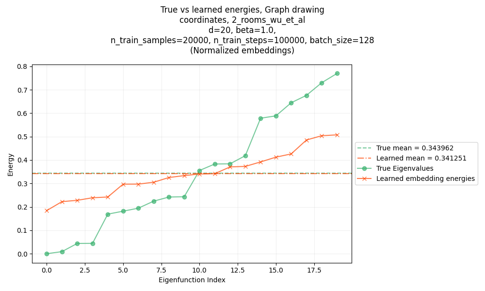
You get the point.
Errata, discussion
High level takeaways
I found this paper helpful for a few reasons that are more abstract than the specific idea itself.
The first is that I’ve learned a ton of cool methods that have their basis in finite dimensional linear algebra. But figuring out how to translate them to continuous functions is often a challenge, or they break down for some reason. This paper basically does that translation, so it’s cool to see it work.
The second is related to the first, but I don’t think I had seen orthogonality of functions enforced this way before. I actually enforced this constraint myself in my recent post on minimizing the GDO with gradient descent, but that was with finite dimensional vectors. They do some clever sampling to enforce it when the vectors are continuous functions.
Another reason is that it takes a somewhat more advanced math idea (the Laplacian) and actually does something with it. This is something I’ve been thinking about for a while and maybe I’ll write something on it soon, but my point is that it’s rare to see something like this actually get implemented and used, so it’s inspiring to see.
Lots of unclear things
The paper is a very cool idea and I enjoyed it a lot. That said, it was pretty unclear in a bunch of parts, where just another sentence or two in the appendix really could’ve cleared things up for me and saved me some time. Maybe some of these are things that one should just be able to know from the context / the other ways wouldn’t make sense, but I dunno.
Is pixels SR… any different than one-hot? Why do the eigenoptions results look bad for them?
This one drove me a bit batty too. Recall that in the Evaluating the Learned Representations section, they experiment with three different SRs: one-hot, coordinates, and pixels. And they show this figure:
Ignore the green line, and whole middle subplot. The thing I’m talking about here is that for the one-hot SR (left subplot), the eigenoptions (red) curve goes to zero for many samples, while for the pixels SR (right subplot), it tapers off to a lousy value.
At first I got similar results (the ones I showed above) and didn’t think much of it. But after changing a bunch of things, I was getting this:
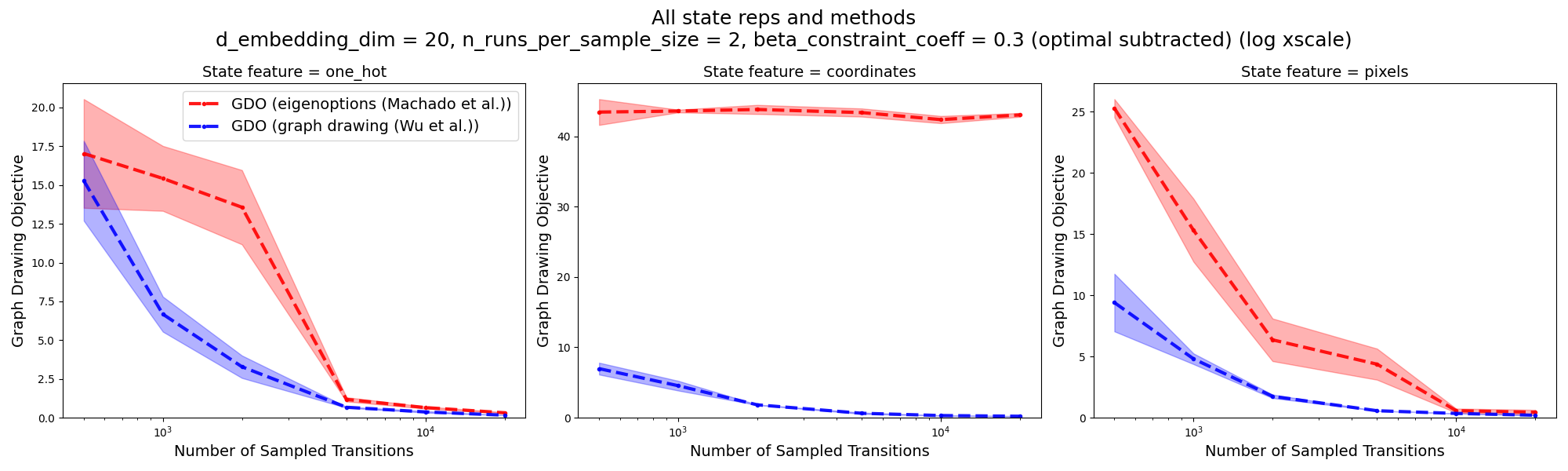
Two big differences:
- For one-hot SR, their method is still better but not MUCH better like it was before
- For pixels SR, eigenoptions also goes to zero gap to optimal, with many samples
After thinking about this a bit more, I’m pretty confused and I’m wondering if they made a mistake (or, much more likely tbh, I did!). Here’s what I’m thinking:
We know that for the eigenoptions method, if the SR is one-hot, then the eigenvectors of the incidence matrix it finds with SVD (given enough samples) will actually be exactly the eigenvectors of the Laplacian.
For other SRs, it should still produce useful eigenvectors (provided there are enough features, unlike with the coordinates SR), but they won’t be literally the eigenvectors of the Laplacian. So I assumed that’s what was going on with the pixels SR.
But, the incidence matrix it uses is formed only from the difference in SRs for the transition states; i.e., transition $(s, s’)$ adds a row $\psi(s’) - \psi(s)$. For one-hot SR, transition $(s_i, s_j)$ would look like:
\[\begin{aligned} t_{ij} &= \psi(s_j) - \psi(s_i) \\ &= [0, 0, \dots, 0, \underbrace{1}_{j}, 0, \dots, 0, \underbrace{-1}_{i}, 0, \dots, 0 ] \end{aligned}\]For the pixels SR, they say:
A image state representation contains $15$ by $15$ RGB pixels with different colors representing the agent, walls and open ground.
It doesn’t matter, but I used $g = (1, 1, 1)$ for the ground, $w = (0.5, 0.5, 0.5)$ for the walls, and $a = (1, 0, 0)$ for the agent. However… if we write out the states and transition above for this SR, we get:
\[\begin{aligned} \psi(s_i) &= [w, w, \dots, w, g, \underbrace{g}_{j}, g, g, \dots, g, \underbrace{a}_{i}, w, \dots, w ] \\ \psi(s_j) &= [w, w, \dots, w, g, \underbrace{a}_{j}, g, g, \dots, g, \underbrace{g}_{i}, w, \dots, w ] \\ \\ \Rightarrow t_{ij} &= \psi(s_j) - \psi(s_i) \\ &= [0, 0, \dots, 0, 0, \underbrace{a - g}_{j}, 0, 0, \dots, 0, \underbrace{g - a}_{i}, 0, \dots, 0 ] \\ &= (a - g) \cdot [0, 0, \dots, 0, 0, \underbrace{1}_{j}, 0, 0, \dots, 0, \underbrace{-1}_{i}, 0, \dots, 0 ] \\ \end{aligned}\]This is the same as the one-hot SR, just with a constant $(a - g)$ factor! Since that’s for literally every since row, it can be factored out of the $\Psi$ matrix and it should also give the same eigenvectors.
So basically… I can’t imagine why it’d behave differently than the one-hot, which is also what I saw in the results.
Unfortunately, I don’t remember what exactly I was doing differently when I was getting those earlier results that looked like theirs…
That said, I have a guess – at some point I realized that while np.linalg.eigh returns eigenvalues in ascending order, np.linalg.svd returns them in descending order. When we calculate the SVD of the incidence matrix, $T = U \Sigma V^\intercal$, and take the first $d$ columns of $V$ to use as the PVFs, naively taking the first $d$ would give much worse results. Additionally, there’s another possible pitfall – for $N$ transition samples ($N > m$, where $\psi(s) \in \mathbb R^m$), $T$ has shape $N \times m$, there are $m$ singular values, and $V$ has shape $m \times m$. However, depending on the SR, $m$ can be bigger than the number of states, which means there are many zero singular values. For one-hot SR, $m$ is exactly equal to the number of states, but for pixels SR, there end up being many zero singular values. Therefore, when selecting the $d$ columns, I think we also need to take the $d$ smallest nonzero ones, or else we’ll be using a bunch of invalid eigenvectors.
Samples vs steps?
Relatively minor, but: they’re a bit unclear about the data they’re training the learned embeddings with. In the Evaluating the Learned Representations experiments (section 5.1), the x-axis is “number of samples” and they say in the appendix that their method is trained for 100k training steps, so that’s pretty clear.
But for the representation learning for reward shaping, they say:
We pretrain the representations for $30000$ steps (This number of steps is not optimized and we observe that the training converges much earlier) by Adam with batch size $128$ and learning rate $0.001$.
I take that to mean 30k training steps, like the 100k above. But what’s the actual number of samples? I just assumed it was a large number like the max number of 20k in the previous section, but again, it’d be nice to tell us that.
What do we do with the eigenoptions method when $d < m$ ?
Okay, maybe I’m missing something really obvious here, but one detail that was pretty unclear to me (and would’ve been really helpful to say explicitly!) is this:
for the eigenoptions method, they form an incidence matrix $T$ of shape $N \times m$ (by stacking rows of $\psi(s’) - \psi(s)$ for transitions $(s, s’)$), and then calculate the SVD $T = U \Sigma V^\intercal$ of it. They then use the columns of $V$ as PVFs $e_i$ (in Machado et al’s terminology), and to find the $i$th embedding for a state $s$ with SR $\psi(s)$, say $f_i(s) = \psi (s)^\intercal e_i$. So to calculate a $d$-dimensional embedding, we just use the first $d$ columns of $V$.
However… $V$ has shape $m \times m$. So for the coordinates SR we have $m = 2$, and I think there are effectively only two PVFs for $V$, and therefore only two embeddings we can make. So… huh? How are we supposed to evaluate this for $d = 20$, like in their figure?
I’m not sure, but I think what they do is effectively tack on an extra $d - m$ columns of random values, if needed, to make sure there are enough PVFs. You kind of need to do this if you want to embed in $d$ dimensions; if you don’t, well, the GDO will definitely be smaller but it’s not a good comparison.
The question is where to slap on those extra columns. We could just do it after the embeddings $f_i$ are found, before they find the principal $d$ directions of the embeddings. However, we could also add the extra columns to the PVFs (i.e., columns of $V$). This makes the most sense to me, but maybe it’s wrong for some reason. I tried both with the coordinates SR, and they’re both about equally lousy anyway.
Why do they use multi-step transitions?
As I mentioned in the reward shaping section, there they use multi-step transitions. Without going too deep into it, the generalization of the weights $w_{ij}$ to the continuous case is basically a kernel function $D(u, v)$ that tells us how much states $u, v$ are “connected”; basically, we can say they’re connected if they transition between each other, which makes sense intuitively if you picture all the states as nodes in a graph.
But they do the multi-step version (in some experiments), which means that $D(u, v)$ will “connect” states that may not have direct transitions between them. I think I get what’s happening, but I just don’t understand the motivation for it. It seems like it could have a bunch of important implications – for example, I suspect the difference in $D(u, v)$ between different policies gets magnified, if you consider multi step transitions. It’s also a harder requirement, since the single step version only requires $(s, s’)$ transitions, whereas the multi step version needs at least segments of trajectories.
Using a different $\delta_{jk}$ value to “control the scale of L2 distances”
In the appendix D.2.1, for the GridWorld experiments for the Laplacian Representation Learning for Reward Shaping, they say:
For the approximate graph drawing objective (6) we use $\beta = 5.0$ and $\delta_{jk} = 0.05$ (instead of 1) if $j = k$ otherwise $0$ to control the scale of L2 distances.
That’s the orthogonality “target” in the constraint. But… what? I see that it’ll make the norm of each eigenfunction $f_i$ smaller, and I guess that’ll decrease the L2 distances when we calculate $\Vert \phi(s) - \phi(g) \Vert$. But is there any reason to not just scale $\phi$ after learning? It also seems like a very strange hack that undercuts the method. How would we know what’s a good $\delta_{jj}$ value for a different, unknown environment?
Wrong eigenoption terminology?
In the appendix, while describing how they do Machado’s baselines, they say:
Implementation of baselines. Both of the approaches in Machado et al. (2017a) and Machado et al. (2017b) output $d$ eigenoptions $e_1, \dots, e_d \in \mathbb R^m$ where $m$ is the dimension of a state feature space $\psi : S \rightarrow \mathbb R^m$, which can be either the raw representation (Machado et al., 2017a) or a representation learned by a forward prediction model (Machado et al., 2017b). Given the $d$ eigenoptions, an embedding can be obtained by letting $f_i(s) = \psi(s)^\intercal e_i$. Following their theoretical results it can be seen that if $\psi$ is the one-hot representation of the tabular states and the stacked rows contains unique enumeration of all transitions/states $\phi = [f_1, \dots, f_d]$ spans the same subspace as the smallest $d$ eigenvectors of the Laplacian.
Not a big deal, but I’m pretty sure they don’t mean what Machado et al call eigenoptions, since those are… options 😛 I’m pretty sure they basically mean the PVFs, given that they use the same notation $e_i$, and the PVFs also get combined with the state reps to form eigenpurposes in that paper. But it’s also a bit confusing since they use $\phi$ for the whole embedding here, while in the eigenoptions paper, $\phi$ is just the state rep.