The quadratic form of the graph Laplacian and finding eigenfunctions with gradient descent
Last time
Last time, when I reviewed some basics of the Laplacian and did a few little experiments with it, I mostly focused on it through the lens of diffusion, since that’s a common use case for it, and it’s pretty helpful for gaining intuition.
I looked at the eigenfunctions of the Laplacian of a 1D bounded region/chain as the special functions that are shaped such that under diffusion, the heat at each point spreads to its neighbor in a perfect balance so that the function’s shape remains the same, and only its magnitude changes (as an eigenvector must). In my eye, that viewpoint was considering them as the fundamental basis functions they are, and how they behave under diffusion, but not really as “solutions” to anything (other than the obvious of the eigenvalue equation $L v_k = \lambda_k v_k$ itself).
Today I’m gonna look at it from a different viewpoint, one that’s closer to the original reason I started looking into this. Specifically, something they’re the solution to, and why that’s useful. However, these different viewpoints really are all connected in a cool way.
The quadratic form and spring energy
A quick refresher on the basics of the (graph) Laplacian:
- we have a graph of $n$ nodes
- we have nonnegative, symmetric weights $w_{ij}$ between nodes $i$ and $j$
- we assume we have an adjacency matrix $A$ for this graph, with entries $w_{ij}$, and zeros on the diagonal
- the degree matrix $D$ comes directly from $A$, and then the Laplacian matrix is $L = D - A$
- we’ll consider functions $f \in \mathbb R^n$, which essentially assign a value to each node
Okay!
Today we’re gonna be looking at a specific expression, $f^\intercal L f$. I’ll motivate it further down, but first let’s write it out in terms of the weights of $A$ and the function $f$.
With the above notation, if you write out $Lf$, you get:
\[\begin{aligned} L f & = \begin{bmatrix} \sum_{j} w_{1,j} & -w_{1, 2} & -w_{1, 3} & \dots & -w_{1, n} \\ -w_{2, 1} & \sum_{j} w_{2, j} & -w_{2, 3} & \dots & -w_{2, n} \\ \dots \\ \dots \\ \dots \\ -w_{n,1} & -w_{n, 2} & -w_{n, 3} & \dots & \sum_{j} w_{n,j} \\ \end{bmatrix} \begin{bmatrix} f_1 \\ f_2 \\ \dots \\ f_n \\ \end{bmatrix} \\ \\ & = \begin{bmatrix} f_1 \sum_{j} w_{1,j} - \sum_{j \neq 1} w_{1, j} f_j \\ f_2 \sum_{j} w_{2,j} - \sum_{j \neq 2} w_{2, j} f_j \\ \dots \\ \dots \\ \dots \\ f_n \sum_{j} w_{n,j} - \sum_{j \neq n} w_{n, j} f_j \\ \end{bmatrix} = \begin{bmatrix} \sum_{j} w_{1,j} (f_1 - f_j) \\ \sum_{j} w_{2,j} (f_2 - f_j) \\ \dots \\ \dots \\ \dots \\ \sum_{j} w_{n,j} (f_n - f_j) \\ \end{bmatrix} \end{aligned}\]we can combine the sums because $w_{k, k} = 0$, so $\sum_{j \neq 1} w_{1, j} f_j = \sum_j w_{1, j} f_j$.
So then $f^\intercal L f$ gives:
\[\begin{aligned} f^\intercal L f & = \begin{bmatrix} f_1 & f_2 & \dots & f_n \end{bmatrix} \begin{bmatrix} \sum_{j} w_{1,j} (f_1 - f_j) \\ \sum_{j} w_{2,j} (f_2 - f_j) \\ \dots \\ \dots \\ \sum_{j} w_{n,j} (f_n - f_j) \\ \end{bmatrix} \\ \\ & = \sum_i f_i \sum_{j} w_{i,j} (f_i - f_j) \\ & = \sum_{i, j} f_i w_{i,j} (f_i - f_j) = \sum_{i, j} s_{ij} \end{aligned}\]If we pair up the terms $s_{ij}$ and $s_{ji}$, we get:
\[\begin{aligned} s_{ij} + s_{ji} & = \underbrace{f_i \textcolor{orange}{w_{i,j}} (f_i - f_j) + f_j \textcolor{orange}{w_{j,i}} (f_j - f_i)}_{\textcolor{orange}{w_{i,j} = w_{j,i}}} \\ &= w_{i,j} [f_i (f_i - f_j) + f_j (f_j - f_i)] \\ &= w_{i,j} (f_i - f_j)^2 \\ \end{aligned}\]So! We finally get the “spring energy” for a function $f$:
\[E(f) = f^\intercal L f = \sum_{i, j} w_{ij} (f_i - f_j)^2\]I think I’m missing a factor of $1/2$ somewhere? YOLOOOOO
So, what’s the intuition here? I already called it the “spring energy”, and it obviously has the form of the elastic potential energy. So if we view the meaning of the function $f$ as assigning a position $f_i$ to each node $i$, $E(f)$ is a measure of the potential energy of the graph, if node $i$ and node $j$ are connected by a spring with stiffness constant $w_{ij}$. This is also called the “quadratic form” because… ya know.
What does this do to the $k$th eigenfunction $v_k$? $E(v_k) = v_k^\intercal L v_k = v_k^\intercal \lambda_k v_k = \lambda_k$. So the energy is just the eigenvalue!
This is another view (i.e., in addition to the heat diffusion perspective) of what the eigenfunctions of $L$ are: they’re the mutually orthonormal functions that minimize the “spring energy” $f^T L f$, given weights $w_{ij}$.
- The first eigenfunction $v_1$ is the constant one, which has $f_i = f_j$ for all, and therefore $E(v_1) = \lambda_1 = 0$
- The second eigenfunction $v_2$ must be orthogonal to it, and will have the next smallest energy $\lambda_2 > 0$ possible, and so on, for the other eigenfunctions
We can imagine finding each next eigenfunction by saying “while being orthogonal to all the previous node arrangements, find an arrangement of the nodes that gives the lowest energy” (see below).
Maybe this is obvious to anyone else, but I think it’s worth saying because it feels a bit weird: the function values are positions along a 1D axis. For example, if we plot the some of the eigenfunctions of a 1D chain from last time:
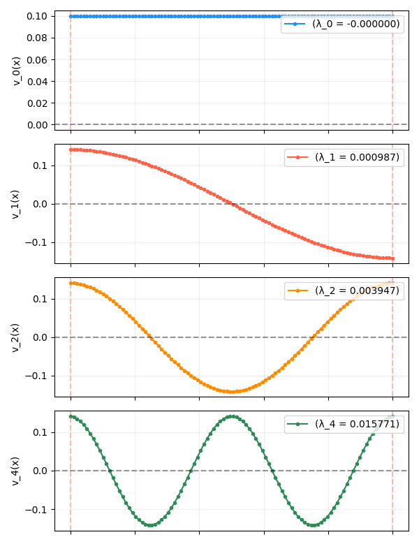
When it’s plotted like this, it’s easy to inaccurately picture them as “heights” along an axis, but really, you should mentally be horizontally squashing each of the curves above against the y-axis, which is the 1D axis the positions are actually on. For example, the 2nd eigenfunction above (in red) looks like:
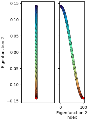
This gives a sense of what they actually look like:
- The first eigenfunction (blue), the constant one, is where all the nodes have the same position. This makes sense, because obviously if you had a bunch of points connected by springs that wanted to minimize the distance between them, they’d all squeeze to the same point, giving zero displacement and $E = 0$.
- The next eigenfunction (red) looks pretty close to a straight line, but it’s actually not. We can see why if we pretend it starts as an actual line centered at zero and think about what would happen to it given the objective we know the eigenfunctions minimize: all the nodes want to move closer to each other while maintaining orthogonality to the other eigenfunctions (and maintaining a unit magnitude). In this case, the only eigenfunction so far is the constant one, so orthogonality with that is already satisfied since it’s symmetric around zero.
- However, it also wants to move the points closer together to minimize the energy $f^\intercal L f$. If we consider the node exactly in the middle, it only has two connections to other nodes, which are at equal distances, and therefore exert an equal force in opposite directions, and therefore has no net force. In fact, this is currently the case for all the non-edge nodes. However, if we look at one of the two edge nodes, it feels the attraction force to its one neighbor, and so it (and the other opposite edge node) can move in a bit. This decreases the total energy, while still maintaining orthogonality to the 1st eigenfunction. If we imagine stepping this forward many times until it settles, this unbalanced force at the edges eventually works its way in, distorting the shape slightly into the sine shape we see.
- The next (orange) and all following eigenfunctions “loop back” to cover part of the 1D space that other nodes already occupy (for example, there are two nodes both at $y = 0$, the horizontal dashed line):
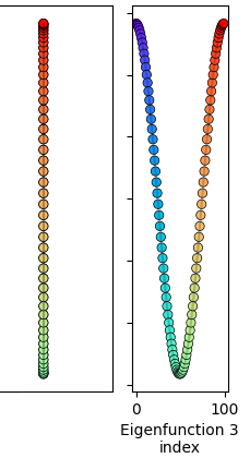
This might seem like it’d be really undesirable in terms of energy, but keep in mind that each node only feels the spring forces from its immediate neighbors, and as far as it’s concerned, the other nodes at that position are relatively far away in terms of the actual adjacency matrix.
Above I said that we can imagine finding each next eigenfunction by requiring: “while being orthogonal to all the previous node arrangements, find an arrangement of the nodes that gives the lowest energy”. I actually got a lot of intuition by doing exactly this, which is what I do below!
Finding eigenfunctions with gradient descent
If the eigenfunctions minimize the energy while being orthogonal to them, we should be able to start from any function and find them via gradient descent.
The objective is clear enough, the energy $E(f)$, but how do we enforce the orthogonality constraint? You can get as fancy as you want with constrained optimization, but at the end of the day a lot of it comes down to “add a penalty term to the objective for how much a candidate solution is violating the constraint”.
In this case, if we have eigenfunctions $v_0, v_1, \dots, v_m$, then $f$ being orthogonal to them means $f \cdot v_k = 0$ for all of them. That’s what we want, so the constraint violation is simply $(f \cdot v_k)^2$. If we call $V_m$ the matrix that has the first $m$ eigenfunctions as its columns, then we get the full objective by just adding the constraint with a coefficient $\beta$ to the energy:
\[J(f) = E(f) + \beta \cdot \|V^\intercal f\|^2\]Note that if we naively calculated $\nabla_f J$ here, $f$ would… immediately shrink to zero for all eigenfunctions. So we actually have the extra constraint that $\vert f \vert^2 = 1$. However, that one is easy to enforce without adding another constraint, I just renormalize so $f \leftarrow f / \vert f \vert$ after each gradient step.
I actually did two versions of this, which I’m calling “sequential” vs “simultaneous”. The difference is that for sequential, I find the eigenfunctions… sequentially, meaning I only optimize one function at a time. For simultaneous… well, you’re a smartypants, you can probably guess.
The difference between them actually turned out to be very interesting and I definitely learned some practical things, so let’s look at them… sequentially.
Sequential optimization
For sequential, the previously found eigenfunctions are frozen, and only the current function is being updated. The previously found ones are passed in for the orthogonality constraint in the objective, but they’re constant.
This one turned out to be really easy! Here it is slamming it for the first few eigenfunctions:
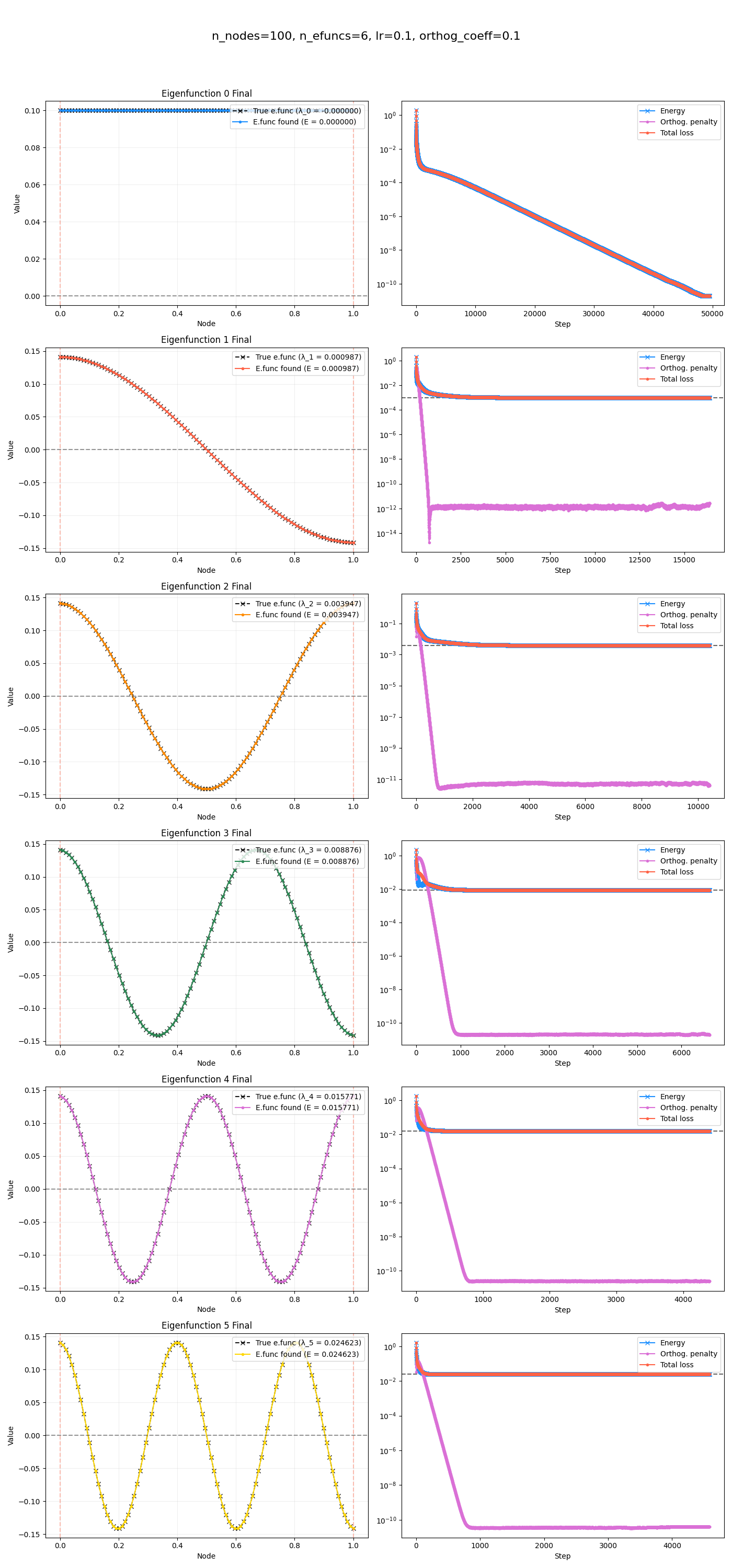
In the left column are the optimized eigenfunctions (in color) and the true eigenfunctions (black); you can see they’re basically exact. The legend also shows the spring energy for each of them. The right column shows the loss terms for each eigenfunction’s optimization; I have it stop when the loss hasn’t decreased for some steps.
It just worked really easily, I basically didn’t have to mess with any parameters or anything. You can see I’m using $\beta = 0.1$ there, but I think it’d prob work with a range of them. And I think this makes lots of sense:
- The first eigenfunction doesn’t have any previous eigenfunctions to be orthogonal to, so its objective is just $E(f) = f^\intercal L f = \sum_{i, j} w_{ij} (f_i - f_j)^2$. This is a super duper convex problem and you can see how fast the loss drops. $\nabla_f E = L f$.
- The second eigenfunction now has the orthogonality constraint with the first eigenfunction in its objective, but this is just another linear term, $\nabla_f (v_1^\intercal \cdot f)^2 \propto v_1 v_1^\intercal f$ in the gradient.
Not much more to say there.
Simultaneous
The sequential method worked easily, but it feels a bit like cheating; for most applications it’d be ideal to find them all at the same time.
To find them simultaneously, if we want to find $m$ eigenfunctions, instead of the variable being a single “column” vector $f$, it’s now the matrix $F$ composed of $m$ vectors as its columns (as if we stacked each of the $f_i$ side by side). The objective is basically the same:
\[J(F) = E(F) + \beta \cdot \|F^\intercal F\|^2\]Note that because we’re finding all the eigenfunctions at the same time, there are no previous eigenfunctions to be orthogonal to; they all have to learn to be orthogonal to each other at the same time, so the $V^\intercal f$ term becomes $F^\intercal F$. As before, after every gradient step, I normalized each of the columns of $F$ separately.
The problem
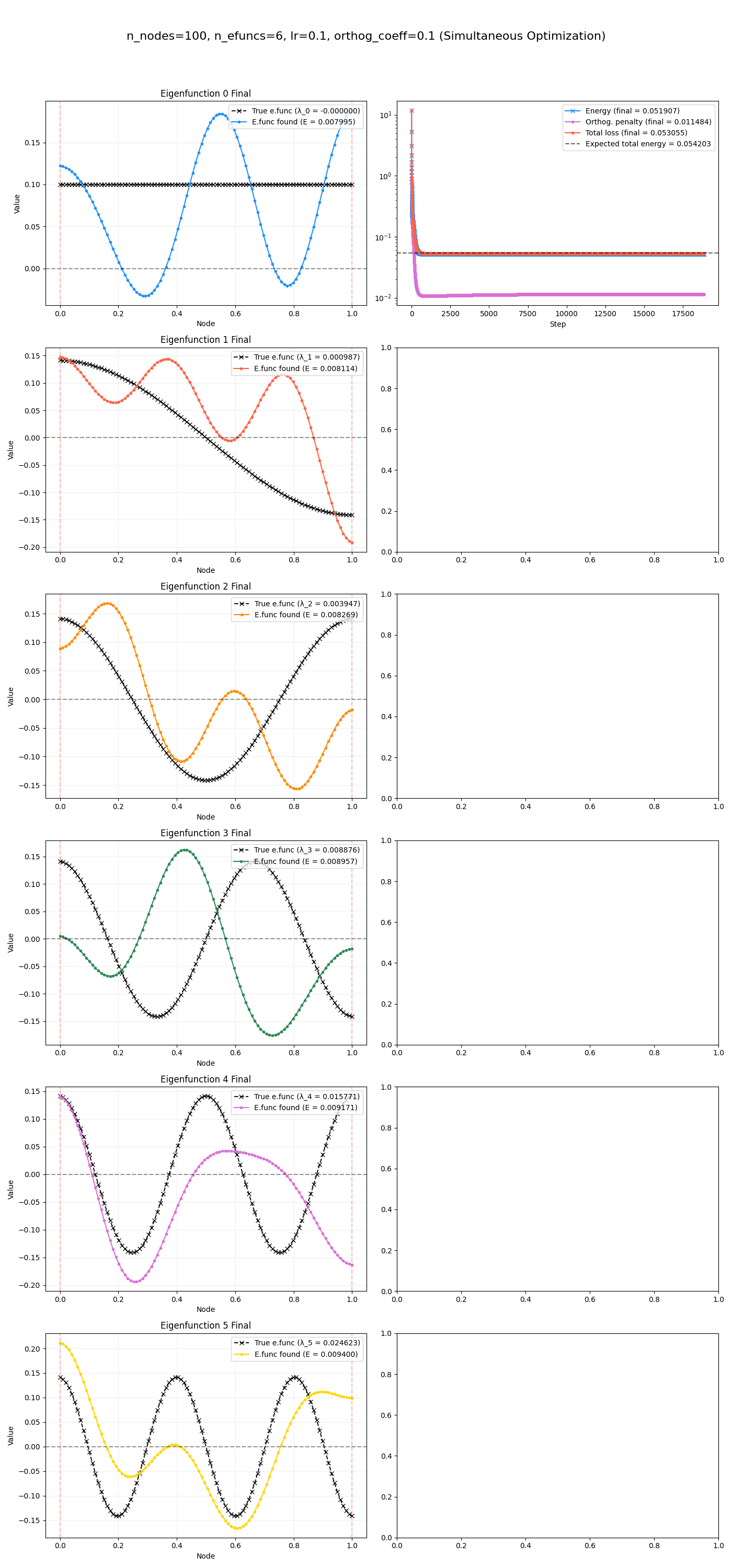
Here’s where I had a good learn! I ran it, saw the loss dropping, but the plots like this:
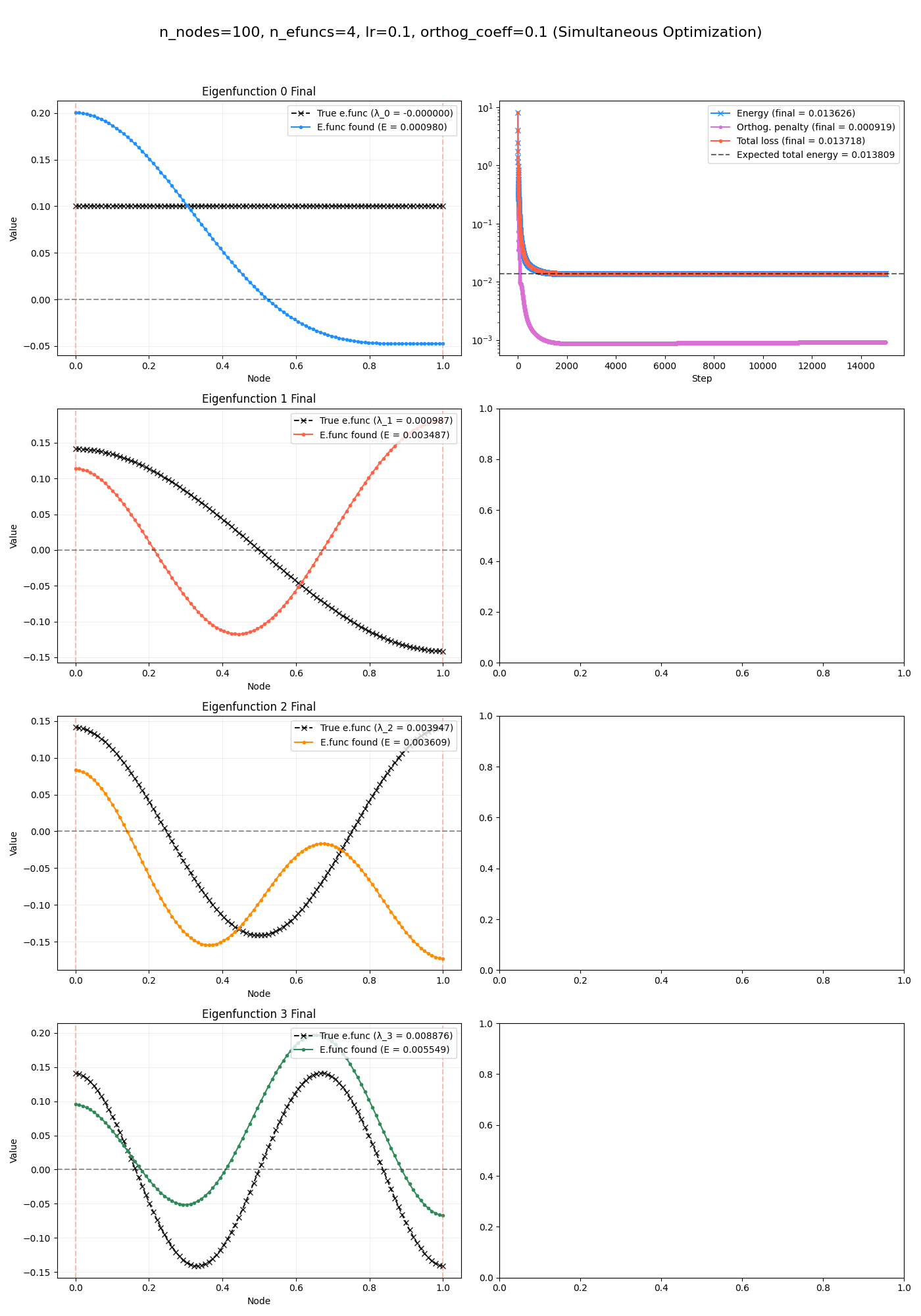
(now there’s only one loss curve, in the upper right plot, because they’re done at the same time so there isn’t a loss curve for each.)
This was pretty confusing to me and I was banging my head against the wall for a while:
- it clearly hasn’t found the eigenfunctions
- (but… they kind of look like the true ones a little, right? curves of similar shapes?)
- however, in the upper right axis, I have the expected true energy (horizontal dashed line), and the $E(F)$ loss term (blue curve) plotted, with their values in the legend:
- expected energy: $0.013809$
- final for loss term: $0.013808$
- these are basically the same! So the functions it has found are very low energy, and in fact are as low as the actual eigenfunctions would be…
- maybe the orthogonality constraints are getting violated, for example if the coefficient for it was too low? That would allow multiple functions to occupy lower energy functions that aren’t fully orthogonal, allowing the total energy to be artificially lower.
- but, the orthogonality penalty curve (pink) is really low in both of the cases above…
- and, the fact that the total energy is nearly exactly the same as the expected energy seems like a pretty big coincidence! If it’s less constrained and that causes the energy to meaningfully drop, there’s no reason it’d stop at that energy.
Basically, the total energy is as low as it should be and the constraint penalty says that it is being satisfied! So how can the solution not be the eigenfunctions? I thought we said that they were the orthogonal functions with the lowest energies!
The answer can be seen by looking at the value of the objective if our solution $F$ could written as $F = V R$, where $V$ is a matrix with the eigenfunctions $v_k$ as its columns and $R$ is an orthogonal matrix:
\[\begin{aligned} J(F) = J(VR) &= E(VR) + \beta \cdot \|(V R)^\intercal (VR)\|^2 \\ &= (VR)^\intercal L (VR) + \beta \cdot \|V^\intercal R^\intercal R V\|^2 \\ &= R^\intercal (V^\intercal L V) R + \beta \cdot \|V^\intercal V\|^2 \\ &= (R^\intercal R) E(V) + \beta \cdot 0 \\ & = E(V) \end{aligned}\]it’s the same as the energy for the actual eigenfunctions! I.e., the objective is invariant to orthogonal rotations within the span of the first $m$ eigenfunctions.
This is how we could find a solution $F$ that has the same energy as the true eigenfunctions, while also being mutually orthogonal – it’s as if we found the first $m$ eigenvectors we were searching for, and then rotated them all. Importantly, it’s invariant to rotations within that subspace of the first $m$; remember that there are $n$ eigenfunctions and if we rotated it to have components from those others, then the total energy would change. This is why I said above that the functions found “kind of looked like” the true eigenfunctions: they were linear combos of only them. I.e., they didn’t have sharp changes or high frequency components.
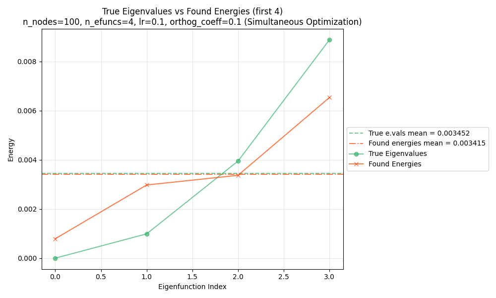
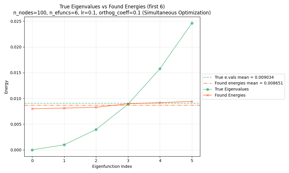
I still had one question though. Alright, the total energy is equal. But we said that the eigenfunctions are special because of their lowest energies. We know we don’t have them exactly, so what is going on with the individual energies?
To make a long story short, the $m$ true eigenfunctions have total energy $\sum_i^m \lambda_i$. Our $m$ found ones also have this total energy, but we know that none of them actually has the lowest energy $\lambda_1 = 0$. Therefore, its lowest energy must be higher, but since the total energy is the same, another found function must have lower energy than the corresponding true eigenfunction!
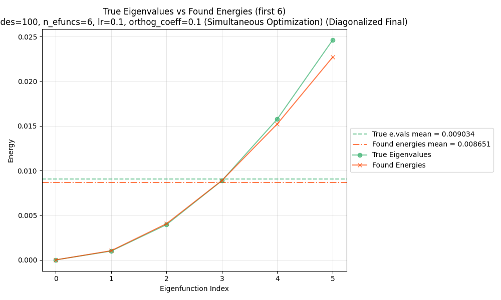
We can see this by plotting both the found and true energies for each function, by their corresponding indices:
and for 6:
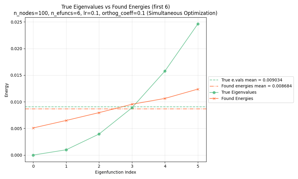
You can see that for both, the mean energy across the eigenfunctions (horizontal dashed lines) is the same. However, in both cases, the first few/lowest energy functions are lower for the true eigenfunctions. For the higher indices, this difference has to be made up, and the found eigenfunctions actually have lower energy.
Super interesting IMO, and lots to think about. A good lesson in there: I spent a long time thinking that my optimization was broken and finding the wrong thing, but in reality I just didn’t realize what it was truly optimizing for.
Anyway, how do we fix it? There are two solutions, one kind of cosmetic and one actually solving the problem.
Fix number one: cosmetic
The “cosmetic” one is simplest, and is just a fix we can do at the end. If we find a solution $F$ that’s a rotation of the $m$ first eigenfunctions $V$, $F = VR$, we can use the Rayleigh-Ritz method. We want the eigenfunctions for $L v_i = \lambda_i v_i$. We have $F \in \mathbb R^{n \times m}$, which has orthonormal columns. We instead set up the eigenvalue problem for the matrix $F^\intercal L F$: $(F^\intercal L F) u_i = \eta_i u_i$. Then, $\tilde v_i = F u_i$ are the “Ritz vectors”, approximations to the real eigenvectors.
Modifying the notation from wiki slightly to match mine:
If the subspace with the orthonormal basis given by the columns of the matrix $F \in \mathbb R^{n \times m}$ contains $k \leq m$ vectors that are close to eigenvectors of the matrix $L$, the Rayleigh–Ritz method above finds $k$ Ritz vectors that well approximate these eigenvectors.
This might feel like cheating: we’re just gonna solve an eigenvalue problem? why go through all this trouble if we can just do that in the first place, directly for $L$? The answer is that we should view the number of data points/nodes, $n$, as being large, so $L$ is a huge matrix we don’t want to do an eigenvalue problem for. But the point of the method above is that $F^\intercal L F$ is actually a $m \times m$ matrix, so that’s reasonable for $m \approx 10$.
So basically, at the end, we can just do this. Here are some ones found, and their energies for each function:
And here they are after that final diagonalization:
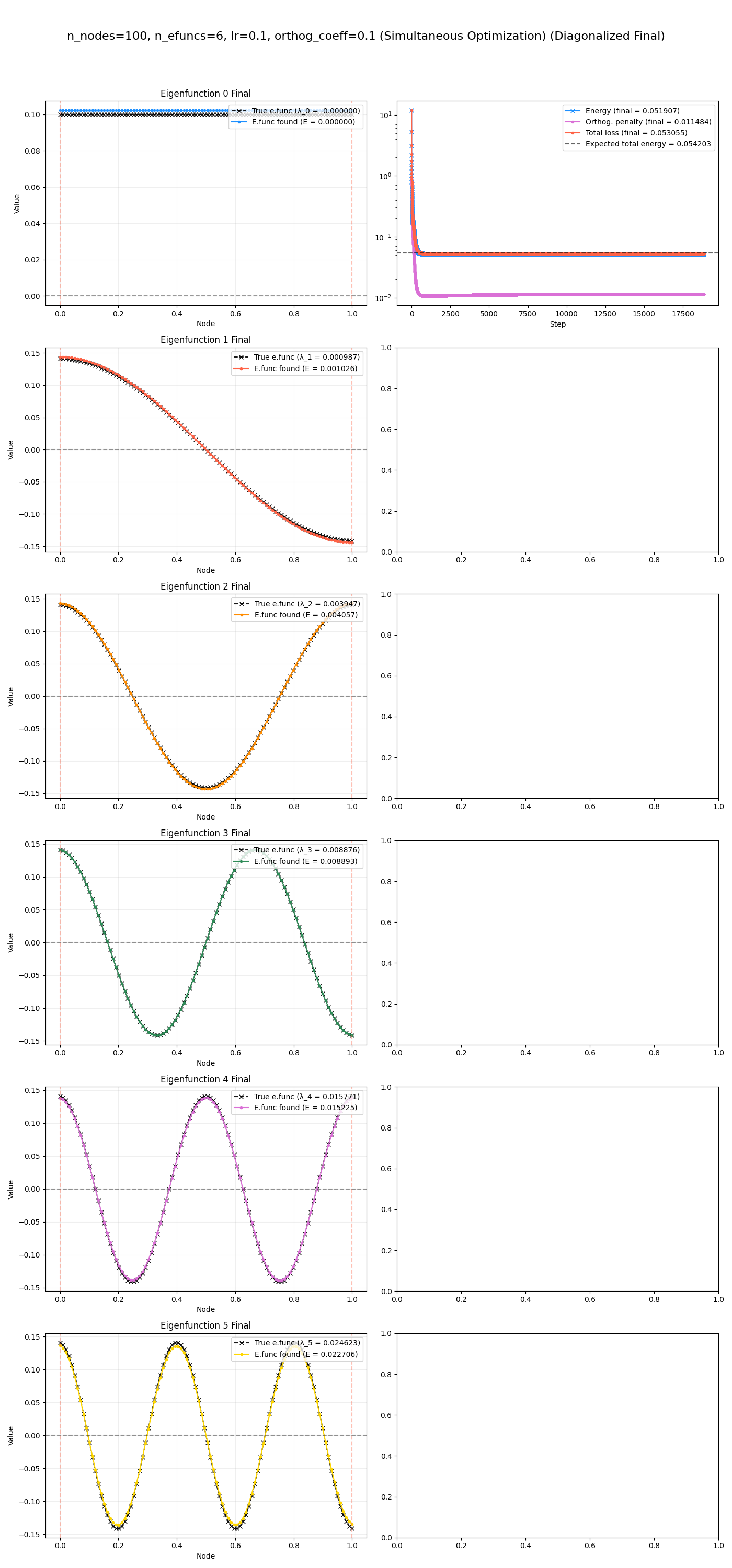
Yeeeeerp, it slams it pretty easily.
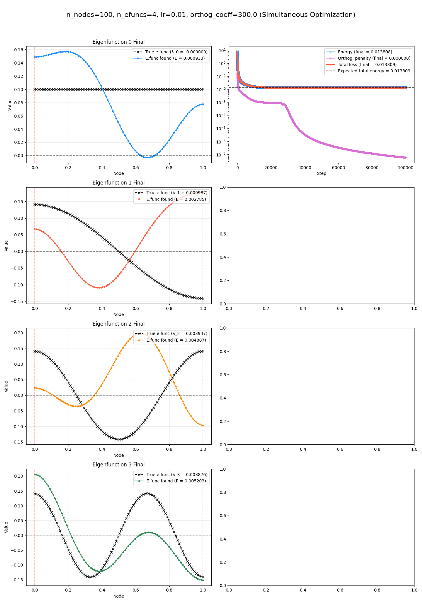
Fix number two: enforced diagonalization
The other method is trying to enforce this during optimization. The math is pretty similar actually. We know that for $V$, the energy matrix $V^\intercal L V \in \mathbb R^{m \times m}$ (i.e., what we sum/reduce to get $E(V)$) is diagonal with the $\lambda_i$ on the diagonal. In contrast, our found solution $F$ has the same $E(V) = E(F)$ once you reduce it, but because it’s a rotation of $V$, it’s all mixed up and has off-diagonal terms in $F^\intercal L F$.
So basically: we add another constraint penalty term. If we’d like $F^\intercal L F$ to be diagonal, the penalty term can be the off-diagonal part of $F^\intercal L F$, i.e. $F^\intercal L F$ minus the diagonal part of $F^\intercal L F$. We square that difference, and make its sum reduction the penalty.
This… was not as easy. In the plots below, I’m not doing the cosmetic final rotation step I mentioned above; I want to see how much the off-diagonal constraint is automatically giving the correct eigenfunctions.
Here’s $m=3$:
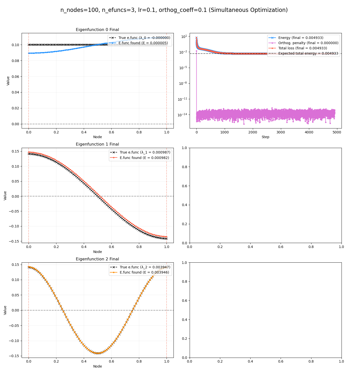
and $m = 6$:
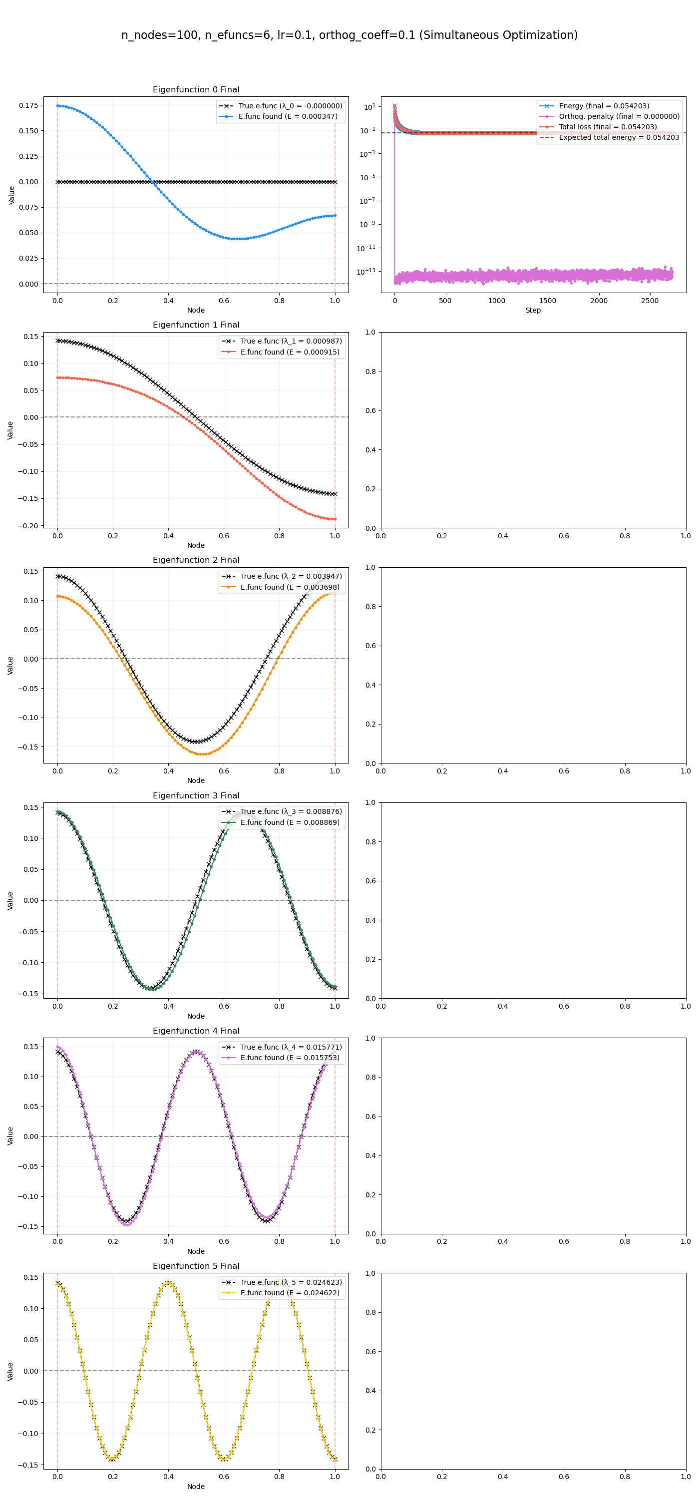
you can see that they’re kind of working, but have some errors. In fact, they seem to work better for the higher energy eigenfunctions, which I wouldn’t have predicted. But I think this makes sense – a slight error in them results in a higher relative error, compared to the smaller energy eigenfunctions, which actually have a tiny energy error even when they’re somewhat far off.
Regardless, I’d like to get it working better sometime.
Well, I didn’t quite get to what I hope to in this post, which is actually using the quadratic form for something, namely graph drawing. That’ll have to be for next time. See ya then!