Alrighty, this post is gonna be mostly for myself, reviewing some basics around the Laplacian operator. I’ll try and keep it real loose, Phil style. To temper your expectations, read it as a slightly more put together view of some notes. I’m reviewing this stuff because the graph Laplacian came up in a few interesting papers that I’ll touch on in the future. At the end I’ll have some pretty plots and gifs, as usual.

Oooh! Pretty!

A few questions I want to answer are:

What’s the Laplacian?
What’s the graph Laplacian?
How are they connected?
What’s the intuitive significance of a function being harmonic?
What does the Laplacian do to a function?
What do the eigenfunctions of it represent, intuitively?

What’s the Laplace operator?

Bluntly: the divergence of the gradient of a scalar function $f$:

\[\Delta f = \nabla^2 f = \nabla \cdot (\nabla f)\]

More helpful intuition from Wikipedia:

Informally, the Laplacian $\Delta f (p)$ of a function $f$ at a point $p$ measures by how much the average value of $f$ over small spheres or balls centered at $p$ deviates from $f (p)$.

In Cartesian coordinates,

\[\Delta f = \sum_i \frac{\partial^2 f}{\partial x_i^2}\]

So to first order, we can think of it as the curvature.

Diffusion, harmonic functions, and equilibrium

If $u$ represents a position-dependent density and it’s at equilibrium, and there’s no source or sink anywhere, then if we have a region $V$ with boundary $\partial V = S$, then the net flux through the boundary is zero:

\[\int_S n \cdot \nabla u \ dS = 0\]

Because as much has to be going out as coming into $V$, so the gradients all have to cancel out. The divergence theorem then says:

\[\int_V \text{div} (\nabla u) \ dV = \int_S n \cdot \nabla u \ dS = 0\]

and since this is true for any $V$, the integrands must be zero at all positions:

\[\text{div} (\nabla u) = \Delta u = 0\]

Solutions to $\Delta f = 0$ are called “Harmonic” functions. So that’s kind of one meaning of a harmonic function: it’s a function that’s at equilibrium everywhere. Note: everywhere. You could have the Laplacian of a function be zero at some location, but be nonzero elsewhere.

The vector Laplacian

Above (and usually) we consider a scalar function $f$. But, since you can take the gradient $\nabla A$ of a vector field $A$, you can also take the div of that, or the Laplacian $\Delta A$. In Cartesian coords, this ends up just applying $\Delta$ to each of the components of $A$ separately. I’ll mostly ignore the vector Laplacian.

What does the Laplacian do to a function?

At first glance, this is a bit underwhelming, IMO. Given some operator, I’m used to applying it to a function, and then it transforms/updates the function into another function that’s the same type as the original.

But here, it seems like the short answer is that the Laplacian doesn’t really “do” anything besides for measuring curvature, or measuring “disagreement” between a point and its neighbors (which is the same thing as curvature, pretty much). I.e.,

\[\Delta f(x_0) = \lim_{r \rightarrow 0} \bigg[ \frac{1}{| B_r |}\int_{\partial B_r} f(x)\ dS \bigg] - f(x_0)\]

so if $\Delta f(x_0) > 0$, that means the values of $f$ on the surface of the sphere are bigger, meaning $x_0$ is a local “valley”, etc (IIRC there are two conventions with the sign of the Laplacian, so below I think I dropped one, but this isn’t super important).

I mean, it’s an operator, so it does transform any function into a new function, but the new function doesn’t seem like it automatically represents the “same type of thing” as the original one.

The more useful/intuitive answer is what that sometimes translates to. Intuitively, if $f$ is the amount of heat at each spot, then if $L f(x_0) > 0$, there’s more heat around $x_0$ than at $x_0$, and heat will flow into it. So you could model the evolution of the heat flow by updating the heat at each spot by stepping it forward with $L f(x_0)$:

\[f(x_0^{t+1}) = f(x_0^t) - \epsilon L f(x_0^t)\]

which is pretty much exactly what the heat equation is! And this is basically just the discrete version of the real/continuous version:

\[f(t) = e^{-L t} f(0)\]

That also makes sense in the context of a harmonic function being the system at equilibrium: if you step forward this system, we have $\Delta f = 0$, so it stays the same, as you’d expect in equilibrium.

However, note that this is only true if $f$ follows that equation. In other physical laws (or mathematical models), $\Delta$ behaves differently. For example, with waves, we get

\[\frac{\partial^2 u}{\partial t^2} = c^2 \Delta u\]

which is instead tying it to oscillatory/wave behavior. Since the heat diffusion version is so helpful for gaining intuition, I’ll mostly use it for examples here, but do some other versions in the future.

What’s the graph Laplacian?

I think it makes sense to first go over the graph Laplacian (GL) before going into any more depth.

Briefly, the GL is the Laplacian operator from above, but instead of being applied to functions of position (typically), it’s applied to functions of graphs. I.e., a function gives each node/vertex in the graph a value.

It’s worth mentioning the “discrete Laplace operator” (DLO), in Wikipedia’s terminology. According to them, the DLO is a discrete analog of the continuous Laplacian, just defined on a graph or grid. But importantly, it might be an infinite grid, like a lattice (e.g., with the Ising model).

The “graph Laplacian” (or Laplacian matrix, or any of a million other names) is basically the DLO when there are a finite number of edges and vertices. That’s what I’ll be considering here. But bluntly, we can basically view the GL as a finite discretization of the original Laplacian.

The reason I think it makes sense to go over the GL before going into the other topics is that if we want to actually simulate/program anything (which I do, to gain intuition), I’m not sure you really can use the non-graph Laplacian. I know nothing so take this with a huge grain of salt, but the Laplacian is an operator on continuous functions. I guess we could do symbolic manipulation, but I think ultimately we’ll probably have to sample any continuous function at some points, and once we do that, it’s basically equivalent to the GL.

Notation, assumptions

There are a bunch of versions of the GL, depending on whether the graph is simple, whether it can have negative weights, loops, is symmetric, etc. Since it seems to be the most common, I’ll look at graphs which:

are finite
have symmetric, non-negative weights $w_{ij}$ between nodes $i$ and $j$
are connected (it’s easy to deal with non-connected, but simpler to assume connected for now)

The main piece of info that defines the GL is the adjacency matrix $A$, defining which nodes are connected, and the weights of those connections:

\[A_{ij} = \begin{cases} 0 & \text{if } i = j \\ w_{ij} & \text{otherwise} \end{cases}\]

The degree matrix $D$ is the diagonal matrix with the sum of weights of the incoming edges, for node $i$:

\[D_{ii} = \sum_{j \in N(i)} w_{ij}\]

(where $N(i)$ are the neighbors of $i$)

Then, the GL is just the matrix with entries:

\[L_{ij} = \begin{cases} \text{deg}(i) & \text{if } i = j \\ -w_{ij} & \text{otherwise} \end{cases}\]

Since the diagonal entries of $D$ are basically the row-sums of $A$, we get $L = D - A$.

Understanding the intuition behind $L = D - A$

At first glance, the definition of the GL, $L = D - A$, seems kind of random. How is it connected to the stuff from before?

Remember that:

\[\Delta f(x_0) = \lim_{r \rightarrow 0} \bigg[ \frac{1}{| B_r |}\int_{\partial B_r} f(x)\ dS \bigg] - f(x_0)\]

i.e., it’s difference between the average value of the values of $f$ on the sphere around $x_0$, versus the value of $f$ at $x_0$.

In a graph, we don’t have a “sphere” around a node, but we do have an analog, which is the node’s neighbors. So, if we wanted to write this out for node $i$, calling the value of $f$ at $i$, $f_i$, the difference between $f_i$ and each neighbor value $f_j$ is an average weighted by the edge weights:

\[\begin{aligned} (L f)_i & = \sum_{j \in N(i)} A_{ij} (f_i - f_j) \\ & = \sum_{j \in N(i)} A_{ij} f_i - \sum_{j \in N(i)} A_{ij} f_j \\ & = f_i \sum_{j \in N(i)} A_{ij} - \sum_{j \in N(i)} A_{ij} f_j \\ & = f_i \cdot \text{deg}(i) - \sum_{j \in N(i)} A_{ij} f_j \\ & = ((D - A) f)_i \end{aligned}\]

What’s not quite clear to me is why we have the factor of $\text{deg}(i)$ there. To me, it seems more like the analog of the continuous Laplace operator would be more like:

\[f_i - \mathbb E_{j \in N(i)}[f_j]\]

and I’d think the expectation/average would then have terms like $A_{ij} / \text{deg}(i)$, i.e., with $\text{deg}(i)$ in the denominator instead. Apparently this does exist and it’s called the “random walk normalized Laplacian”, $L_\text{rw} = I - D^{-1} A = D^{-1} L$, but it has some different properties. I’ll hit this in the future.

Connecting the GL to the Laplacian

Allllright, with that out of the way, now we can look at some fun stuff. If we want to simulate the regular Laplacian on some region, we can basically define a graph on a finite number of points representing that region, decide how they should be connected, and then we’ll have the GL for the discretized version.

For example, when we simulate the Laplacian on a 1D, bounded region $[0, a]$ below, we can define the graph as a 1D “chain”, where the nodes are at evenly spaced points starting at $0$ and ending at $a$, and each node is only connected to its immediate neighbors with a weight of $1$ (except for the nodes at the end of the chain; more on that below). With these weights, we get the adjacency matrix, which gives us the degree matrix and the GL.

What are the eigenfunctions of the Laplacian?

There are a few wrinkles here that make this tricky:

being an $L^2$ function or not
the region the function is defined on
being a real or complex function
the boundary conditions (if any)

I mean, they’re all related.

So we’re looking for functions $u$ that have: $\Delta u = \lambda u$ everywhere on their domain.

Unbounded domain

The first issue is that usually when they talk about “eigenfunctions”, like in functional analysis, they specifically want ones that are $L^2$, meaning square integrable over their domain, meaning:

\[\int_\Omega |f|^2 \ dx < \infty\]

So as a simple example, if our domain is $\Omega = \mathbb R^n$, a constant function $u$ does have the property that $\Delta u = 0$, so it seems like it should be an eigenfunction with eigenvalue zero. Similarly, $u(x) = \sin(k x)$ has $\Delta u = -k^2 \sin(kx) = -k^2 u$, so it seems like it’s an eigenfunction. However, in both cases, the integral of their square over $\mathbb R^n$ is infinite, so they’re not $L^2$ and aren’t “proper” eigenfunctions. Instead they get called “generalized eigenfunctions” (I think totally unrelated to generalized eigenvectors a la Jordan chains, etc?).

Something significant here is that you might notice that those generalized ones, the sine for example, have a form that placed no constraints on the value of $k$ – i.e., it could be anything. In contrast, for standard finite vector spaces, we’re used to having only a finite number of eigenvectors/values, that only take on specific discrete values. I guess that’s unavoidable, because they’re finite. But (see below), even for continuous bounded functions, there end up being constraints on those eigenvalues.

So for unbounded $\Omega = \mathbb R^n$, in fact, the only generalized eigenfunctions are $\cos(kx)$, $\sin(kx)$, and linear combos (including complex numbers) of them, and the only true (i.e., $L^2$) eigenfunction of them is the trivial one, zero, and I think we usually don’t count that.

Bounded domain

On the other hand, if the region $\Omega$ is bounded, it’s very different. First we have to establish something that tripped me up for a bit, about boundary conditions. In quantum mechanics we have the classic example of an infinite square well (ISW) defined on $[0, a]$. I want to look at the analogous case for heat diffusion, where instead of the function representing complex probability amplitudes, it just represents the temperature.

For the ISW in QM, it’s common to use Dirichlet boundary conditions, i.e., the function is zero at the edges. In QM, that makes sense because we’re saying the potential outside of $[0, a]$ is $\infty$, so the wave function has zero probability of being there, and we want it to be continuous in space, so it has to be zero at the values $0$ and $a$ as well.

So I initially assumed this when doing the math/simulations and gaining intuition for the heat diffusion case, but quickly made myself confused. The problem is that the Dirichlet BC’s of $f(0) = f(a) = 0$ doesn’t result in the same behavior with heat as it does for the ISW. For the ISW, $f(0) = f(a) = 0$ acts like an infinite barrier that prevents the probability mass from “escaping” the well. In contrast, the same BC for the heat case means that the temperature at those edges is fixed to zero, but that means that for the points immediately adjacent to the edges, they’ll either leak or absorb heat, depending on whether their temperature is above or below zero. Regardless, since the edges are zero, they effectively act as an infinite heat reservoir of temperature zero, so any nonzero heat profile in $[0, a]$ will eventually converge to be all zero.

I guess it’s been a while since I took E&M, because I definitely knew of the solution to the problem here, but I guess I didn’t make the connection. To make the heat analog of the ISW, we instead want to use boundary conditions that specify the value of the derivative of the function at the edges, specifically $f’(0) = f’(a) = 0$. There are a bunch of intuitive ways to see this, but I like to understand it as a device at each edge that perfectly matches the current temperature at that edge. Since it’s the same temperature at the edge as right outside of it, no heat is transferred across the edge in either direction, preventing the “leaking” problem from above. Note that this means that the temperature at the edge can now change (as heat from the region $(0, a)$ moves around), but none will ever leave the edges to the “outside”.

aaaaanyway, solving for the eigenfunctions of this gives us:

\[v_n(x) \propto \cos \frac{n \pi x}{a}\] \[\lambda_n = (\frac{n \pi}{a})^2\]

which are true $L^2$ eigenfunctions. And importantly, the spectrum here is discrete, even though it’s infinite – you only get eigenvalues $(\frac{n \pi }{a})^2$, so it can’t take any old value.

Okay, but what’s the significance of the eigenvectors (in the bounded region / discrete eigenvalues case) ?

Writing the Laplacian as $L$ now and the function as $f$, and the eigenvalues/functions as $\lambda_k, v_k$, the eigenvalue equation is: $L v_k = \lambda_k v_k$ .

I.e., since $v_k$ is an eigenvector, it just scales it by $\lambda_k$. In the typical fashion, we consider what the heat equation from above would do to a single eigenfunction $v_k$, using the matrix exponential:

\[\begin{aligned} f(t) & = e^{-L t} v_k \\ & = [I - Lt + (\frac{Lt}{2})^2 - \dots] v_k \\ & = [I - \lambda_k t + (\frac{\lambda_k t}{2})^2 - \dots] v_k \\ & = e^{-\lambda_k t} v_k \\ \end{aligned}\]

so basically it makes that eigenfunction decay with that exponential coefficient. And then of course the next step is applying it to a linear combination of the eigenfunctions:

\[\begin{aligned} f(t) & = e^{-L t} \sum_k c_k v_k \\ & = \sum_k c_k e^{-L t} v_k \\ & = \sum_k c_k e^{-\lambda_k t} v_k \\ \end{aligned}\]

So there are a few key takeaways here:

Under diffusion, all functions… well, diffuse. However, the eigenfunctions are special, in the sense that as they diffuse, they actually keep the same shape! Because $f(t) = e^{-\lambda_k t} v_k$, and $e^{-\lambda_k t}$ is just a scalar, $f(t)$ always has the shape of $v_k$, and it looks like it’s just shrinking in magnitude.
However, any non-eigenfunction will change shape as it diffuses. If you imagine an initial function that’s a big spike of heat, it’ll spread out and get wider under diffusion. Mathematically, we can understand this because a non-eigenfunction will have a time dependent decay for each eigenfunction component, and they’ll decay separately, changing the relative weights of the different components, and therefore changing the shape.
What does this mean intuitively though? If we imagine each position getting (or giving) some heat to its neighbors, then the eigenfunctions are shaped such that they’re perfectly “balanced” in terms of each position having a net flux that makes it change by the same fraction.
The first eigenfunction, $n = 0$, is special: we have $v_0 \propto \cos 0 = 1$, and $\lambda_0 = 0$. $v_0 = 1$ means that it’s a constant function, and $\lambda_0 = 0$ means that the diffusion coefficient is $\exp[- \lambda_0 t] = 1$. This represents equilibrium!
One more thing is that we know the eigenvalues are all non-negative, with the equilibrium one being zero (with constant eigenfunction), and all the others being positive. So if we consider an arbitrary combination of them, $f(t) = \sum_k c_k \exp[-\lambda_k t] v_k$, determined by the $c_k$ coefficients, then we can see that the equilibrium component will stay at the same magnitude (since it’s just $\exp[0]$), and all other components will decay. And, the higher the eigenvalue, the faster the decay. Those higher eigenvalues have eigenvectors that are more “oscillatory” in space. Since they’re more oscillatory, you can imagine that they have bigger temperature deltas in a given width, which would drive the component towards zero more quickly.

The Laplacian vs the diffusion operator

I’m kind of repeating myself now, but I’ll be really explicit. We were talking about the eigenfunctions/eigenvalues of the Laplacian above, but there’s a bit of a disconnect. Usually with linear operators, we’re used to their higher magnitude eigenvalues being more important and their eigenfunctions being more “dominant” with repeated application of the operator. But above, we saw that the eigenfunction components with higher value eigenvalues actually diffuse faster, and the lowest eigenvalue, $\lambda_0 = 0$, is the one that remains. What’s going on?

We weren’t exactly applying the Laplacian itself when we were diffusing. The actual operator above was $\exp[-L t]$. And because it’s the negative of $L$ in that exponential, that means higher (positive) eigenvalues decay their eigenfunctions faster. Note that both of the operators $L$ and $\exp[-L t]$ have the same eigenfunctions $v_k$, but have different (but related) eigenvalues $\lambda_k$ and $\exp[-\lambda_k t]$, respectively.

One more thing: above I said that we can intuitively see why the “average value at a point compared to its neighbors” interpretation of the Laplacian leads to the heat equation, by looking at a finite-difference of the update:

\[f(x_0^{t+1}) = f(x_0^t) - \epsilon L f(x_0^t)\]

which is the finite-difference version of $f(t) = e^{-L t} f(0)$. Alternatively, you might recognize the finite difference version as the 1st order Taylor expansion of $\exp[-L t]$.

When we want to do this with the GL, we’re not gonna be using a matrix exponential, so we’ll actually use the finite difference version above. This ends up having a matrix analog for the Laplacian vs diffusion operator deal above. If we write the finite difference update equation for a function $f_k$ as:

\[f_{k+1} = f_k - \alpha L f_k\]

you can see that we can pull out $f_k$ and call the resulting operator $T = I - \alpha L$:

\[f_{k+1} = f_k - \alpha L f_k = (I - \alpha L) f_k = T f_k\]

This is the diffusion operator for the GL. It has all the same similarities to the one above: it has the same eigenfunctions $v_k$ that $L$ has, since $T v_k = (I - \alpha L) v_k = (1 - \alpha \lambda_k) v_k$, and similarly, its eigenvalues are different, but kind of “inverted” a little: $\lambda_k \rightarrow (1 - \alpha \lambda_k)$.

Experiments

For all of these, I’ll look at the effect of using the GL for diffusion, on a 1D bounded region, $[0, 1]$. So we’ll have $N$ nodes in the graph. I think because we have an unweighted graph and all we care about are the neighbors, it can be a simple graph, the adj matrix just has zeros and ones, and the degree matrix is just a count of the neighbors.

Finding the eigenfunctions, power iteration

We have the analytic form of the eigenfunctions above. But what if we didn’t?

We want the eigenvectors/values of $L$, but like we saw above, $T$ has the same eigenvectors, so we’ll find the eigenvectors for $T$ instead. I implemented a little power iteration algo to do this, and it ended up being interesting enough on its own that I wrote about it here.

Now I can apply it to the graph Laplacian to find the eigenfunctions for this 1D heat diffusion scenario. How do you know when you’ve found an eigenfunction, though? Well, if you have a pure eigenfunction, applying $T$ will make it still point in the same direction, so the dot product of the post-normalization, post-$T$-application function with the pre-application function should be nearly $1$. Therefore, to check for convergence, we check this error from $1$ and stop once it’s below some threshold.

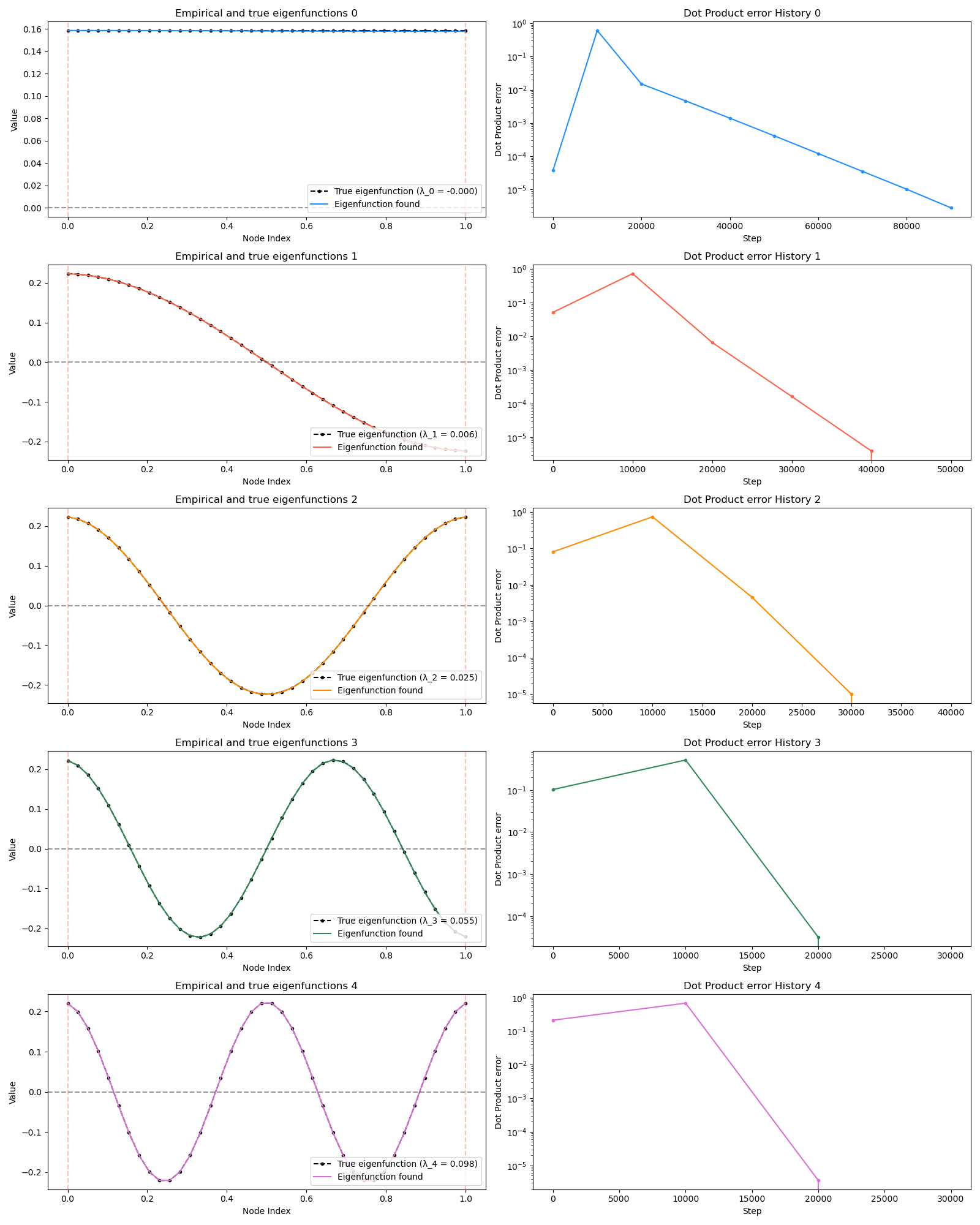
and look at that, it works! In the left column, the true eigenfunctions are the black dots, and the colors are the ones found by this PI process. In the right column is a plot of the error from the ideal dot product, for each eigenfunction.

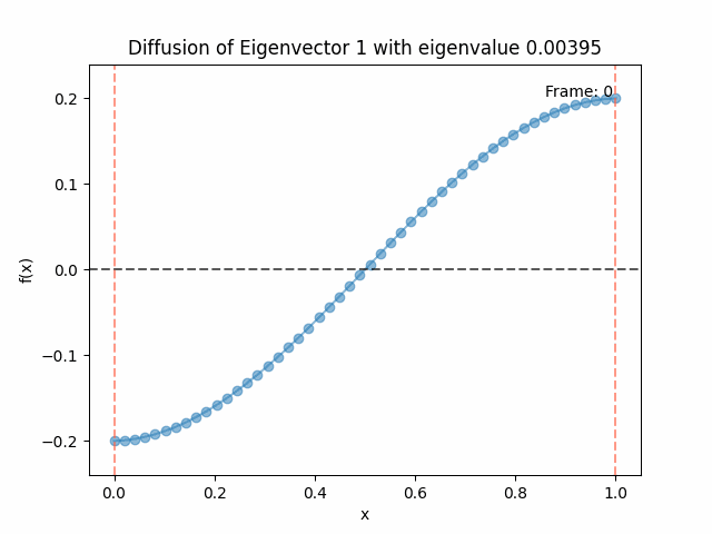
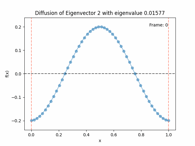
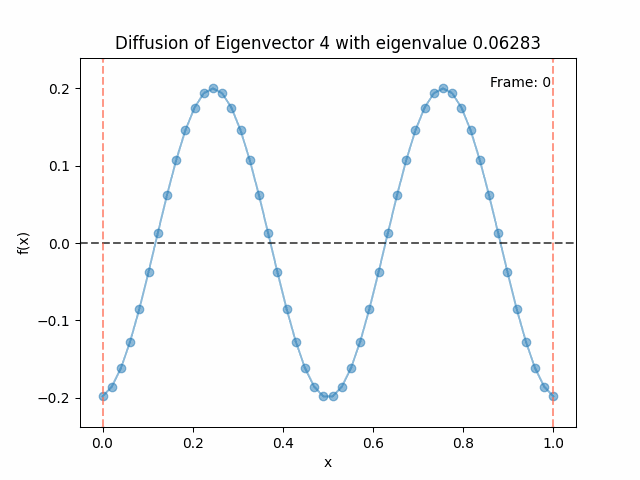
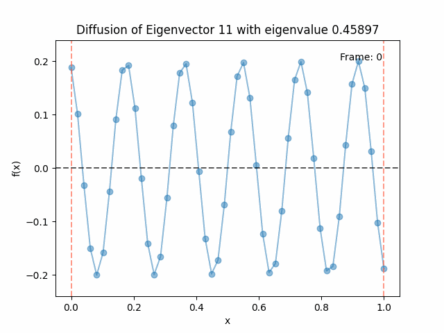
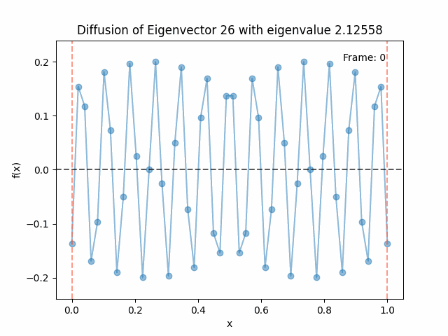
Diffusing the eigenfunctions

Above I mentioned that under diffusion, the eigenfunctions will keep their shape, and just decrease in magnitude. Here we can watch that happen:

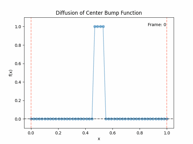
Meanwhile, as above, a non-eigenfunction will change shape as it diffuses:

Also as I mentioned in the eigenfunctions section, the higher eigenvalue (higher “frequency”) eigenfunctions will decay faster, and the $\lambda = 0$ one will be constant. Actually, in the plots above, I had to futz with the diffusion timestep a little between the gifs for the different eigenfunctions. If I used the same for all, then either the higher ones would diffuse way too fast to see much of, or the lower ones would be so slow no reasonably sized gif could show the diffusion for very long. Remember, the decay is with the exponential of the eigenvalue!

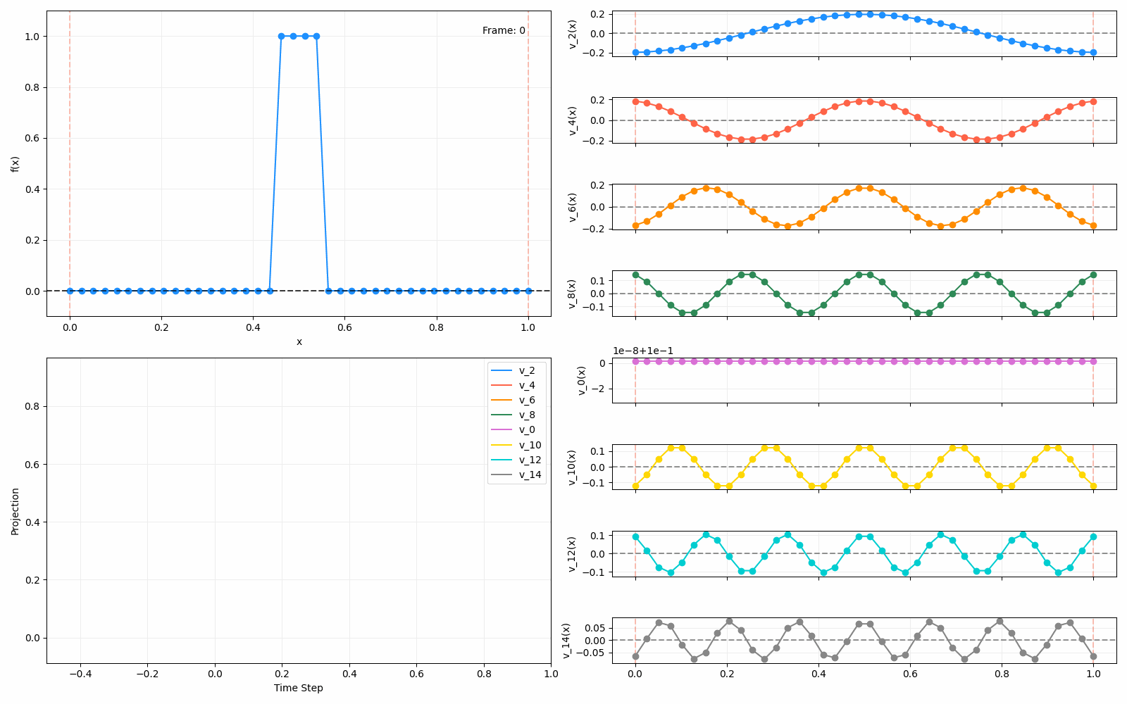
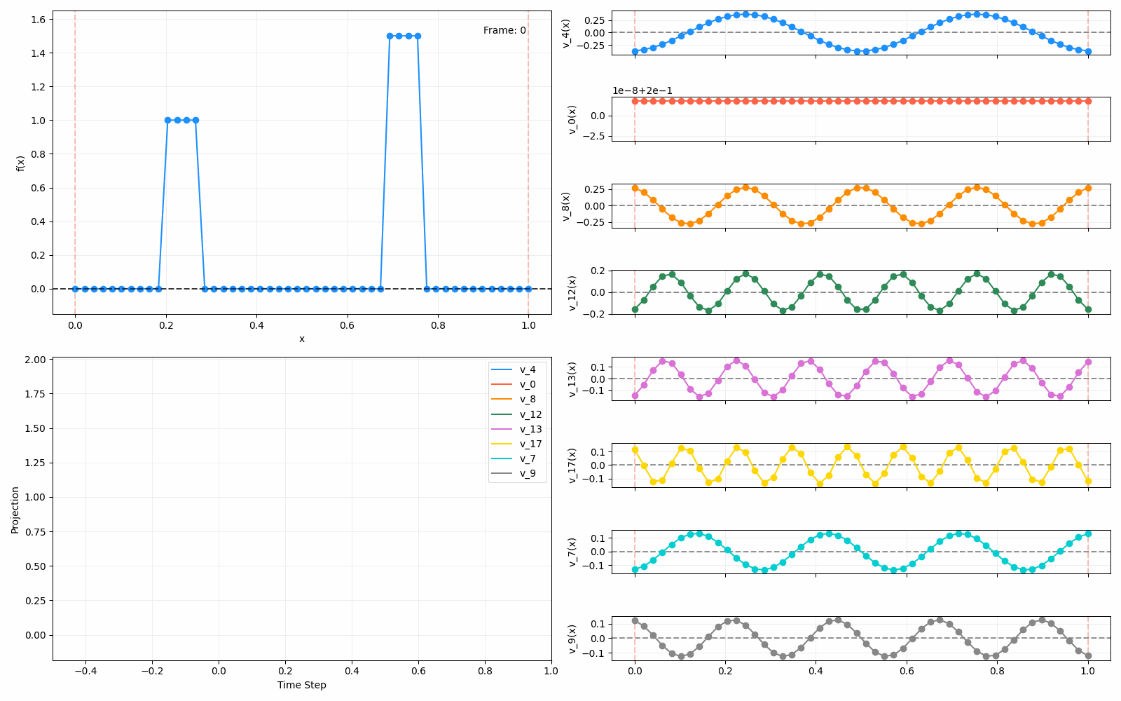
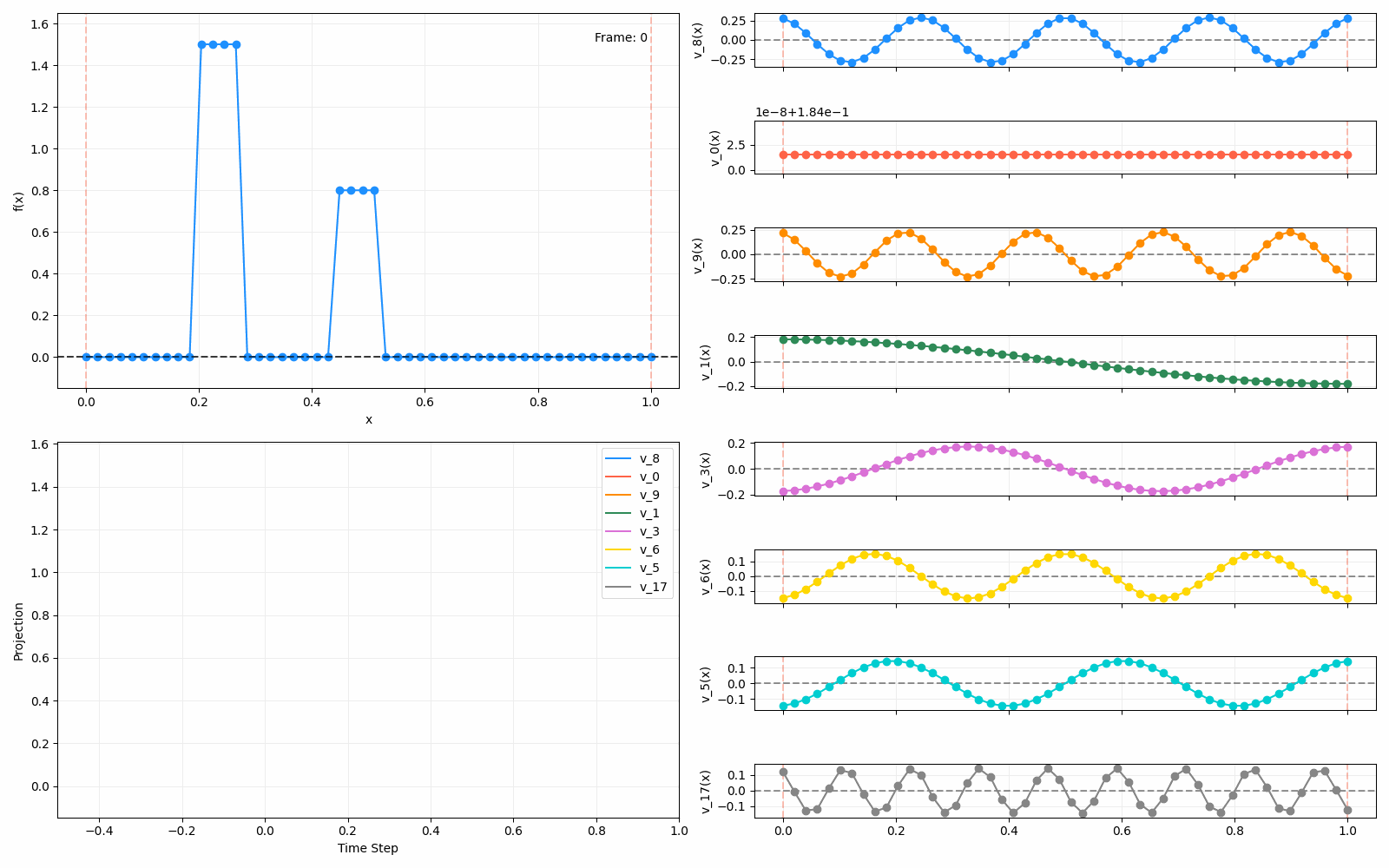
We can put them all together in this gif, where I diffuse that same “bump” function above, but also show the diffusion of its largest eigenfunction components at the same time:

The bottom left plot shows the amplitude of each of them – you can see from that, and just visually on the right how quickly those high frequency/eigenvalue components diffuse away.

For fun, here are two other initial functions:

Anyway, that’s all! This one had a focus on diffusion, which was useful to understand. Next time I’ll be looking at a different interpretation of the Laplacian and its eigenfunctions, which was the original reason I started looking into this. But to be honest, they’re all connected in some fascinating ways.