A fun little aside that I stumbled into while doing another post. This ended up being interesting, and one of those things I only learned from implementing it. I made two stupid mistakes, one a little dumb, and one a lot of dumb. Yeeehaw!

Motivation

Let’s say we have a nice linear transformation represented by a square matrix $A$. Generally, a matrix is fully characterized by its eigenvalues, their multiplicities, and its eigenvectors. Many many things in science and math involving a matrix (i.e., nearly everything) become waaaay easier if you have this info about your matrix.

If you’re doing something small and you want to see the eigen-everything, you can just do e_vals, e_vecs = np.linalg.eig(A) and you’re done.

But what if our matrix is really really big, or we only need the first eigenvector? I just tried np.linalg.eig on a size $10,000 \times 10,000$ random matrix, let it run for like a minute, and then my computer started making the music skip and I frantically hit Ctrl+C to stop it before it crashed my whole machine.

Power iteration (PI) is one method for doing this. PI always lets you find the eigenvector with the largest eigenvalue. But in the case where the matrix is symmetric, the eigenvectors are all orthogonal, and therefore we can find all of them.

Main idea

The idea is that if we take any old vector $f$, it can be expressed as a linear combo of the eigenvectors $v_i$, and applying $A$ to $f$ acts on each of the eigenvectors $v_i$ separately, effectively multiplying them by their eigenvalue $\lambda_i$:

\[\displaylines{ f = \sum_i c_i v_i \\ g = A f = \sum_i c_i A v_i = \sum_i c_i \lambda_i v_i \\ }\]

If we then took the resulting $g$ and normalized it to unit magnitude, we could repeat this. One of the eigenvalues, $\lambda_k$ is the largest, and since that component in the sum is accumulating a factor of $\lambda_k$ for each application of $A$, eventually it dominates the vector and we find that applying $A$ many times results in that eigenvector!

A slightly more intuitive way to see this is explicitly writing out the terms of $f$:

\[f = c_1 {v_1} + c_2 {v_2} + \dots + c_n {v_n}\]

applying $A$:

\[\begin{aligned} A f & = c_1 \pmb{v_1} + c_2 {v_2} + \dots + c_n {v_n} \\ & = c_1 A {v_1} + c_2 A {v_2} + \dots + c_n A {v_n} \\ & = c_1 \lambda_1 {v_1} + c_2 \lambda_2 {v_2} + \dots + c_n \lambda_n {v_n} \\ \end{aligned}\]

and applying $A$ many times:

\[A^m f = c_1 \lambda_1^m {v_1} + c_2 \lambda_2^m {v_2} + \dots + c_n \lambda_n^m {v_n}\]

Hopefully it’s clear that if some $\lambda_k$ was bigger than the others, then for enough applications of $A$, that term would dominate, and we’d have $A^m f \approx c_k \lambda_k^m v_k$. Then, knowing we applied it $m$ times, we could divide $A^m f / (c_k v_k) \approx \lambda_k^m$, and take the $m$th root.

That’s PI, and it should work with any diagonalizable matrix. For symmetric matrices, you can then repeat this process to find the other eigenvectors, but you first have to subtract the projection of the function onto the previous eigenvectors you’ve found: $f - \sum_i \langle f, v_i \rangle v_i$. This effectively takes those eigenvector terms out of the sum above, so that now $A$ only acts on the remaining ones, revealing the eigenvector with the next biggest eigenvalue, etc.

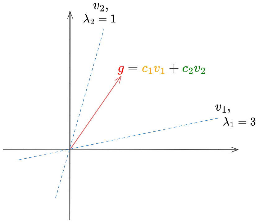
Here’s the first thing I realized, which is a bit embarrassing to be honest. I wanted to test my PI code on a simple 2D operator, so I whipped up a simple non-symmetric matrix, like the one with the eigenvectors/values pictured below, where eigenvector $v_1$ has the larger eigenvalue $\lambda_1 = 3$, and we’ll apply $A$ to the vector $g$.

Drawing 2025-09-02 11.35.32.excalidraw

And it found the first eigenvector easily:

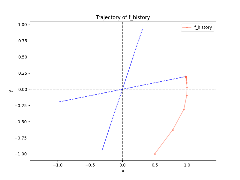
But, going to the 2nd eigenvector, I was confused for a few minutes when my code kept returning the first eigenvector despite subtracting the projection… and here’s my first dumb mistake 🤦

My (incorrect!) thinking was that as long as the matrix is full rank and has linearly independent eigenvectors, subtracting the projection of $g$ on the first eigenvector $v_1$ should “remove” the component $c_1 v_1$, and then PI should lead us to the next eigenvector. I.e., apply $A$ to $g - \langle g, v_1 \rangle v_1$ repeatedly.

This felt right, but it’s wrong. This pic illuminates the problem:

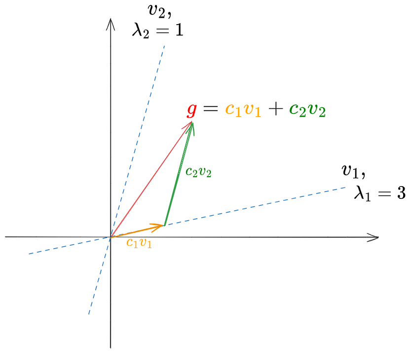
Drawing 2025-09-02 11.22.39.excalidraw

even though $v_1$ and $v_2$ are linearly independent, they’re not orthogonal. Therefore, calculating:

\[\langle g, v_1 \rangle v_1 = \langle c_1 v_1 + c_2 v_2, v_1 \rangle v_1 = c_1 v_1 + c_2 \langle v_2, v_1 \rangle v_1 \neq c_1 v_1\]

you can see that subtracting this from $g$ is not going to remove the $v_1$ component $c_1 v_1$ – it has that extra term in there because $\langle v_1, v_2 \rangle \neq 0$. If you could remove $c_1 v_1$ from $g$, then this process would work… but you can only do that if you know $c_1$, which we don’t know! We don’t know exactly how much of $g$ in the $v_1$ direction comes from $v_1$ itself, as opposed to combinations of the other eigenvectors, which also have components in the $v_1$ direction!

So, that was dumb of me and I should know better by this point, but at least the next one is slightly more interesting. I changed it to a symmetric matrix that necessarily has orthogonal eigenvectors, and ran it. Here it is finding the first eigenvector correctly:

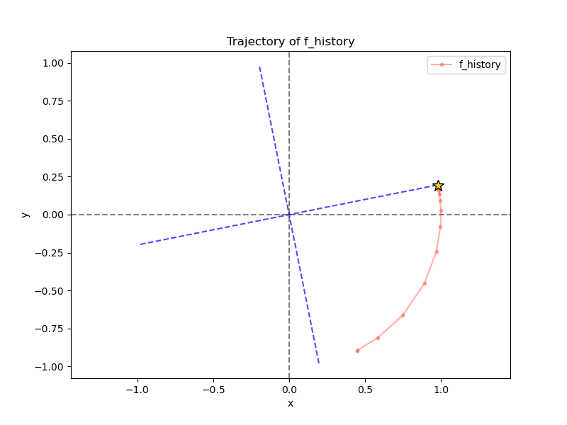
It starts at the red dot, and ends at the yellow star. Whooooo. But looking at the PI trajectory of the second eigenvector:

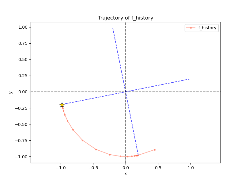
…what’s going on? It immediately jumped to the 2nd eigenvector, but then later went back to the 1st one…

The problem here is that I was only subtracting the projection on the first step. Theoretically, this should be fine! Now that the eigenvectors are orthogonal, if we have $g = c_1 v_1 + c_2 v_2$, then we should have $g - \langle g, v_1 \rangle v_1 = g - c_1 v_1 = c_2 v_2$. Therefore, applying $T$ to $c_2 v_2$ should keep it in the subspace that has no $v_1$ components, and PI should reveal the next biggest eigenvector.

However… numerical precision is a real thing! Subtracting the projection didn’t work fully, so it ended up being $g - \langle g, v_1 \rangle v_1 = \epsilon v_1 + c_2 v_2$, $\epsilon \approx 0$, after that first step. Then, with the subsequent applications of $A$ (without subtracting the projection, because I thought it was gone), the PI process did its thing, and amplified the $v_1$ term until it dominated again! You can actually see this from the pattern of the red dots – after the first one, they’re closely clustered for a while because it’s only amplifying a very small component.

If I instead make it subtract the projection each iteration, we get:

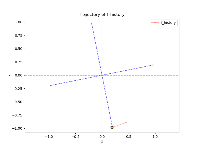
Alrighty! Good to know.

Some patterns and trends

Here are a few things I noticed while poking around! I mainly want to look at the behavior and properties of PI for single $n \times n$ matrices, and then look at the scaling and trends across different sizes.

I’m making an $n \times n$ symmetric matrix $A$ by sampling the elements, and then making it symmetric by setting $A \leftarrow (A + A^\intercal) / 2$.

Uniformly distributed elements

First, here’s an example plot, for an $n = 5$ matrix:

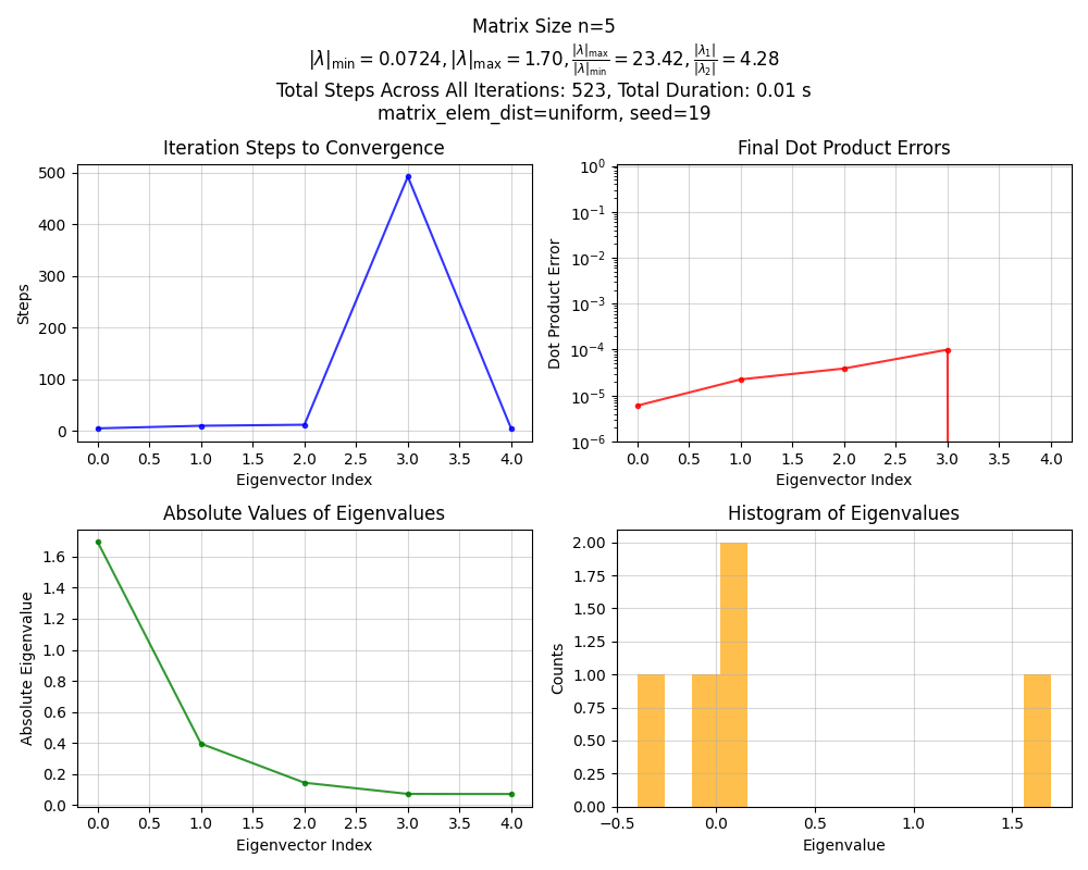
The top left plot shows the number of iterations PI took for finding each eigenvector
The top right shows the final dot product error for each iteration. In this case, the threshold for considering it converged was 1e-4, so we shouldn’t see any values higher than that
The bottom left shows the absolute value of the eigenvalues found, in the order that they were found. Note that they’re of course automatically sorted, since it finds them in decreasing order
The bottom right shows the histogram of these eigenvalues
There’s some other relevant info in the title

Okay, nothing crazy. Now for $n = 100$:

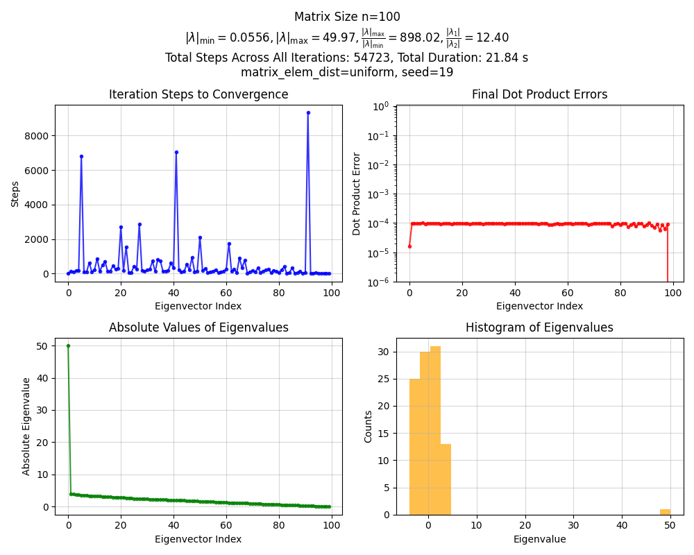
Whoa, that’s weird! The first eigenvalue is huuuge compared to the others. What’s going on?

I (thoughtlessly) first made it generate the matrix $A$ using np.random.rand() (link) for the elements. I wasn’t thinking about it much, but looking at rand(), it’s actually a uniform distribution on $[0, 1)$. Why does this lead to this one huge eigenvalue?

It makes sense if we look at the random variable of the matrix $A$ and rewrite it:

\[\displaylines{ A = \mu \pmb 1 \pmb 1^\intercal + W, \\ \mu = \mathbb E [A_{ij}] = 0.5, \\ W_{ij} \sim \mathcal U [-0.5, 0.5] }\]

We’re kind of writing $A$ in terms of its SVD, where $\mu \pmb 1 \pmb 1^\intercal$ is the first term, and $W$ is all the others. Importantly here, $\mu \pmb 1 \pmb 1^\intercal$ is a rank-$1$ matrix, and $W$ is the sum of all the other rank-$1$ components. You can easily see that the only nonzero eigenvector of $\pmb 1 \pmb 1^\intercal$ is $v = [1, \dots, 1]$:

\[(\pmb 1 \pmb 1^\intercal) v = \pmb 1 (\pmb 1^\intercal v) = \pmb 1 \cdot n = n \cdot v\]

and it has eigenvalue $n$. Therefore, the matrix $\mu \pmb 1 \pmb 1^\intercal$ gives the eigenvalue $\mu n = 0.5 \cdot 100 = 50$ … which is almost exactly what we see! In reality, for finite $n$, $\mu$ isn’t exactly this value, and the largest SVD component actually isn’t exactly $1 1^\intercal$, it has some randomness too, like the $W$ components. But we can see that even for $n = 100$, it’s pretty spot on.

There are two important parts here: 1) this first eigenvalue scales with $n$, and 2) it also scales with $\mu$. But $\mu$ is the mean of the sampling distribution, and it’s only nonzero because of that dang rand() ! So, if we use a zero-centered distribution (like I intended), then this $\mu n$ term goes away, leaving the randomness that gave rise to the other eigenvalues.

Ok, but what about the other eigenvalues? Let’s look at them next.

Normally distributed

Allllright, now let’s just use np.random.normal to generate the matrix. We could just use np.random.uniform(low=-1, high=1.0) to get rid of the positive-mean aspect from above, but I originally intended to use a Gaussian and it’s more typical anyway.

Here’s that for $n = 100$:

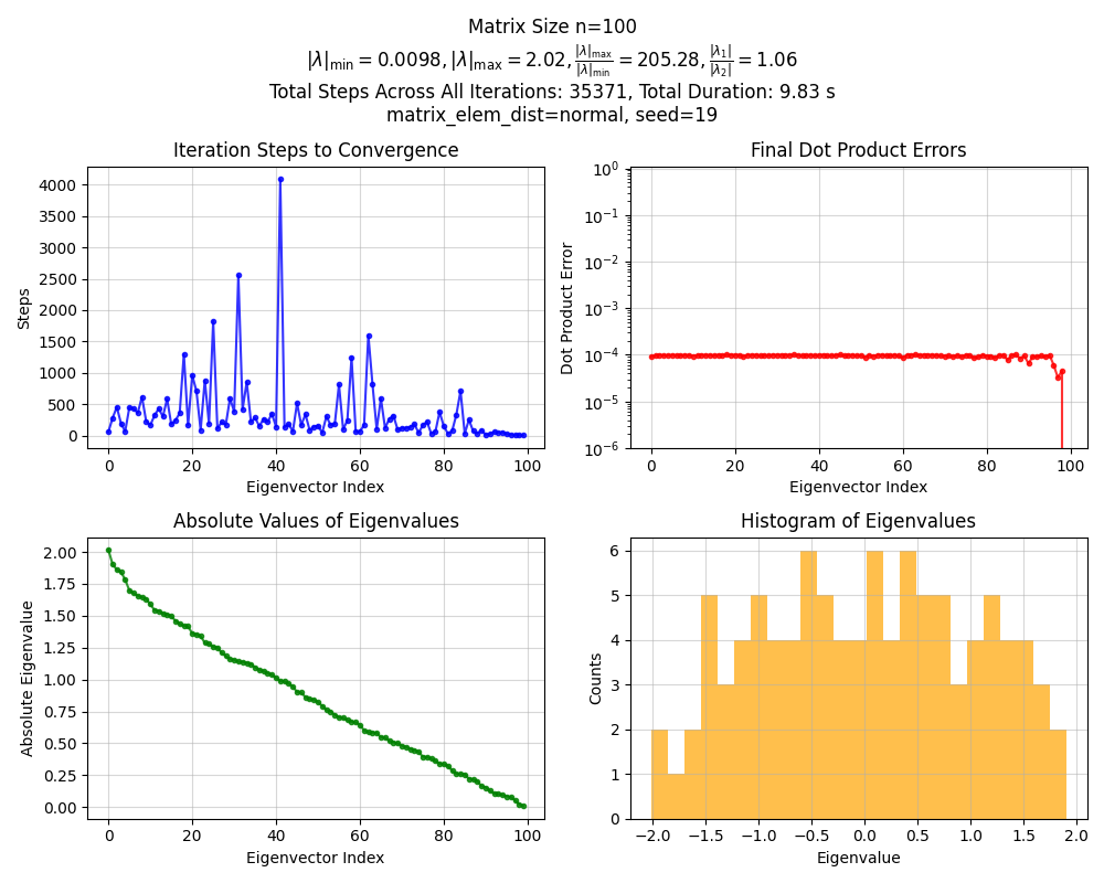
You can see off the bat that the eigenvalues are distributed much more evenly. If you squint at the histogram, it kind of looks… semi circular? It turns out that this is known as Wigner’s Semicircle Law. In short, if we look at random matrices whose elements are sampled from certain distributions (most commonly, independent Gaussian), then the distribution of their eigenvalues approaches that semicircular shaped distribution as the matrix size goes to infinity.

As they mention in the mathworld and this link, this actually applies to many more random matrices than Gaussian ones, including uniform distributions (as long as the matrix is symmetric). I actually scaled the Gaussian matrix $A$ in the above by $\sqrt n$, which is why the eigenvalues are bounded by $[-2, 2]$ (for any $n$), but (I think) in the uniform case above where I didn’t do that scaling, the semicircle distribution bounds would be $O(\sqrt n)$. That explains the qualitative behavior: the “big” eigenvalue was growing as $O(n)$, and the others as $O(\sqrt n)$.

I don’t yet have a good grasp of why the semicircle law works, but this post is already too long so I’m not gonna dig into it today. I’d like to learn more about Random Matrix Theory sometime. Terence Tao wrote a book on RMT, which is probably great if it’s anything like his Analysis books we used in undergrad.

Convergence speed of 1st eigenvector

One more little thing from the above plots: you can see in the title that I added the ratio $\vert \lambda_1 / \lambda_2 \vert$, the (abs) ratio of the first to the second eigenvalues. As they mention in the PI wiki article, this ratio determines the convergence speed (of finding the first eigenvector).

And it intuitively makes sense, right? If we view PI as magnifying the biggest eigenvalue component each iteration, then if the biggest eigenvalue is a lot bigger than the next biggest, it’d amplify the dominant eigenvector more quickly.

According to wikipedia, the convergence speed goes as $\vert \lambda_1 / \lambda_2 \vert^k$, where $k$ is the number of iterations.

If you look at the Gaussian one, you can see that it has $\vert \lambda_1 / \lambda_2 \vert \approx 1.06$. I ran it for 5 seeds and $n = 100$, and the steps to converge the first eigenvector were [59, 526, 72, 389, 237]. In contrast, the uniform one above had $\vert \lambda_1 / \lambda_2 \vert \approx 12$, which makes sense because of that huge first eigenvalue. I also ran it for the same 5 seeds, and its step to converge were: [6, 8, 6, 6, 5]. Way faster! I did a bit of back of the envelope math with those values, and they seem to line up.

Scaling with $n$

Here I’m looking at, for an $n \times n$ matrix as above, how long it takes to find all the eigenvectors. This is definitely not the way you’d want to do this, I’m just curious about it.

I ran it from some sizes in the range [2, 200] because my code is totally unoptimized and it was already being annoyingly slow at the higher end:

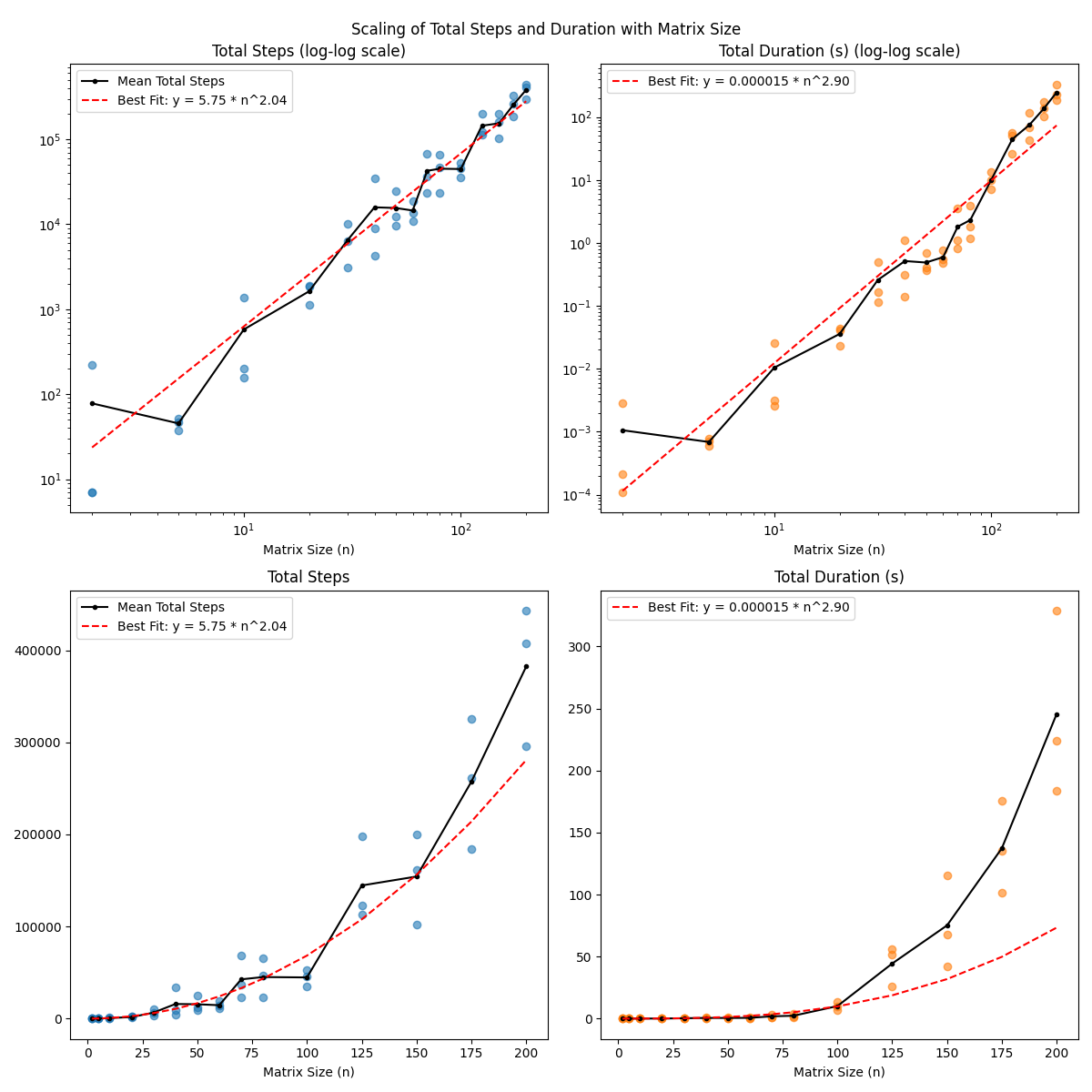
I plotted both the total steps (i.e., the number of PI steps to convergence, summed across all eigenvectors), and the total time duration. I’m guessing the total time duration is more meaningful, since a “step” here involves matrix multiplications/etc, so is obviously doing more computation per step for $n = 200$ than for $n = 2$.

I tried a few different scales, and it looked a lot more linear on a log-log scale (implying a power law equation) than it did on a log-scale (which would imply an exponential equation). This makes some fuzzy, intuitive sense to me; it seems like exponential complexity usually comes from some element of combinatorics, which this doesn’t have.

I think naively, it should be $O(n^3)$ in basic operations, since a single PI step needs $n^2$ for the $A x$ matrix-vector multiplication (the other parts are $O(n)$), and then there are $n$ vectors to find, so $O(n^3)$ total. And maybe it’s coincidence, but the exponent in the right plots is $2.9$!

Errata

So I should go out and use PI to find all the eigenvectors now, right!?

Uhh… probably not. The applications section on WP has some examples where it’s supposedly used, like for PageRank and Twitter’s algo. But my impression is that for most “real” applications, there are fancier methods, some of which they mention. I mean, PI is pretty crude, and it’s really only intended to find the dominant eigenvector. I think if you want to find the others as well, you should probably be using methods for that (like the QR algo or divide and conquer eigenvalue algos).

That’s aside from the actual implementation magic. I only know the teensiest bit about this, but I do know that they’re doing some real creative stuff at the low linear algebra level. One reason is just for performance, but others have to do with a million pitfalls we haven’t even considered here around matrix conditioning, FP precision (like above but way more subtle), numerical stability, etc.

For example, the doc page for np.linalg.eig mentions they use the “_geev” LAPACK routine, which you can see the source for here. I’m sure it’s a bit more readable if you know any Fortran, but it’s still clearly doing more than you’d expect.

An actual use in the wild!

That said: I’ve actually seen it used once in a paper!

I was reading an RL paper I’m a big fan of, “Lipschitz-constrained Unsupervised Skill Discovery”. To make a long story short: they’re training a state embedding $\phi(s)$, but want to constrain it such that:

\[\displaylines{ \forall x, y \in \mathcal S, \\ \|\phi(x) - \phi(y) \| \leq \|x - y\| }\]

I.e.: for a given magnitude of difference between inputs, they want the difference between the outputs to be less than or equal to that (hence the “Lipschitz” in the name).

But of course it’s 2025 so $\phi$ is generally implemented with a big ol’ neural network. To enforce the constraint above as the inputs go through the network, we effectively have to control the slope of all the functions (linear transformations from weight matrices and nonlinearities) that get applied to it. If we can keep the slope (of the function $\phi$ as a whole) always below $1$, then we know that there will never be two points that could break that constraint.

So how do you enforce that? They borrow a technique from another paper, “Spectral Normalization for Generative Adversarial Networks”. For the NN’s nonlinearities, ReLU has slopes of either zero or one, so that’s easy. But a given weight matrix $W$ could be anything, and can certainly increase the magnitude of a vector $x$ it’s applied to. The “spectral radius” or “spectral norm” $\sigma(W)$ of a matrix $W$ is the maximum ratio $|W x| / |x |$ for any input $x$; it’s effectively the most it can possibly increase the magnitude of any vector.

I bet you see where this is going! The (absolute value of the) largest eigenvalue of $W$ is basically this. So if the spectral norm can be calculated for each $W$, it can be used to adjust the effect of $W$ and keep the Lipschitz constant of the network as a whole below one. And of course, they use PI to do that.

There are a few interesting details here. First is how they use it. There are actually two papers, this one and another, that use basically the same idea. In this one, they approximate $\sigma(W)$, and then when doing a forward pass, just divide the resulting vector by $\sigma$, which ensures its magnitude will stay below one. I.e., the weights of $W$ themselves are unconstrained, and we just do extra math to account for that. But in the other version, I believe they use $\sigma$ for a penalty, which actually does change the weights.

Another issue you might have immediately bring up is… they’re doing PI… inside a NN? for each layer? many times, during optimization? didn’t I just show a bunch of plots where it sometimes takes many steps to converge??

They address this in the appendix:

If we use SGD for updating $W$, the change in $W$ at each update would be small, and hence the change in its largest singular value. In our implementation, we took advantage of this fact and reused the $\tilde u$ computed at each step of the algorithm as the initial vector in the subsequent step. In fact, with this ‘recycle’ procedure, one round of power iteration was sufﬁcient in the actual experiment to achieve satisfactory performance. Algorithm 1 in the appendix summarizes the computation of the spectrally normalized weight matrix $\bar W$ with this approximation. Note that this procedure is very computationally cheap even in comparison to the calculation of the forward and backward propagations on neural networks. Please see Figure 10 for actual computational time with and without spectral normalization.

One round! That sounds a bit crazy. But there are probably some mitigating factors. The first is that like they say, they’re starting off with a good vector for estimating it. So provided it doesn’t change drastically between updates, the last vector direction the PI yielded will probably still be good. They also don’t necessarily need to find the spectral norm exactly; they really just want to control it from blowing up over the course of many layers. So it might not be so bad if they’re a little off and it’s slightly bigger than one.

The last interesting thing is that $W$ is not generally square the way we’ve been assuming! That’s not actually a problem for computing the SN $\sigma(W) = |W x| / |x |$, since you just compute the norm in the input and output spaces. But, in the stuff above, we’ve been assuming that $A$ was square, meaning that the output size is necessarily the same as the input size, meaning that we can easily apply $A$ repeatedly. So how would you do that with non-square $W$? You basically just go “back and forth” between the input and output spaces by applying $W$ to an input space vector $v$, normalizing the result and calling it $u \leftarrow W v / |W v |$, and then doing the same in the other direction, using $W^\intercal$ and calling it the new $v \leftarrow W^\intercal u / |W^\intercal u |$.

Wow. What a crazy journey we’ve been on here, mannn. I think we’ve both learned a lot. Crazy.