Eigenpurposes, eigenbehaviors, and eigenoptions, oh my!
Approaching the present
In a bunch of recent posts on the Laplacian (🐙, 🦣, 🐷, 🦜), I’ve been reviewing basics and concepts, and then looking at a couple older papers involving the Laplacian. Those were all interesting, but very old news by now. Today we’re gonna look at a more recent work in the same vein, “A Laplacian Framework for Option Discovery in Reinforcement Learning” (2017). It’s a very fun and clever idea, and definitely influential on later work.
The big ideas
This paper really follows from Mahadevan’s Proto value functions paper, so check out my post on it if you’re not familiar. The PVF paper uses the PVFs mostly as a basis to construct other value functions (VFs).
One of the main ideas of the Eigenoptions paper is that we can use PVFs not only as a basis, but also to define interesting tasks. PVFs tend to capture task-independent structure of the environment, like all those pretty pictures you can see in the PVF post. The idea here is that if we use a given PVF to define a reward, that reward should also capture some fundamental structure of the environment. Then, we can train a policy to optimize for this reward.
The PVF captures some meaningful structure of the env, but it’s pretty passive – it’s really just a “shape”, a scalar function. The clever idea of this paper is turning that PVF into a behavior that reflects that structure!
As the paper’s name suggests, their motivation for this is option discovery, i.e., using those PVF policies as options. There was tons of work on options back in the day, but my impression is that these days they tend to be viewed as a kind of ugly hack. Regardless, they show that the options can be useful for exploration.
Another idea from the paper (I think it’s from this?) is to take collected env transitions and use some basic but clever linear algebra to approximate the eigenfunctions of the Laplacian. That lets you find them without having to build an adjacency matrix, which is basically infeasible for real state spaces.
Eigenpurposes, eigenbehaviors, eigenoptions
Assume we have a PVF $e \in \mathbb R^m$ and state representation $\phi(s) \in \mathbb R^m$. Then, we can define a reward function for it:
\[r^e(s, s') = e^\intercal (\phi(s') - \phi(s))\]They call this reward function an “eigenpurpose”, because it’s giving the agent a “purpose”, and it’s an eigenfunction. Very cute.
(For initial understanding, you can assume $\phi(s)$ is a one-hot vector, i.e. $\phi(s) \in \mathbb R^{ \vert S \vert}$ where $\vert S \vert$ is the number of states, and likewise assume $e \in \mathbb R^{ \vert S \vert}$ too. They do this for exposition and some of the results in the paper, and I do it here too, but it’s good to have the more general form in mind since a one-hot state rep isn’t really practical.)
Given an eigenpurpose, there’s some optimal VF and policy for it. And aren’t you surprised to learn that they call the optimal policy for an eigenpurpose an “eigenbehavior”? Super kawaii~
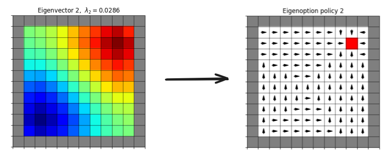
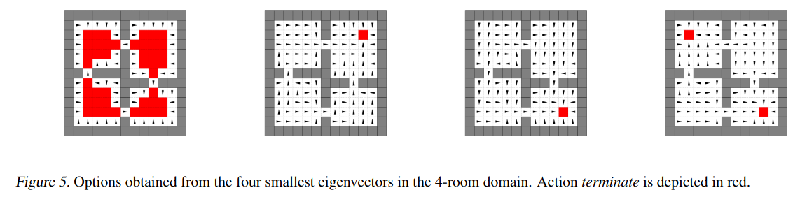
To make this concrete, here’s a figure from their paper:
You can see that the arrows of the eigenbehavior are basically following the gradient of the PVF on the left.
To turn a policy (in this case an eigenbehavior) into an (eigen)option, you need to define termination states for it, where the option would stop and the high level controller would take over again. They define the termination states for an option as the states where the eigenbehavior has… achieved its eigenpurpose, meaning it can’t get more (cumulative) rewards for that eigenpurpose. This basically happens when it’s at a local maximum of the VF for that eigenpurpose. They give the agent a “terminate” action that it can do when it reaches those states. You can see it marked in red in the figure above.
A few examples
Okay, let’s get our hands dirty to give a sense of what’s happening here. Here are the steps I’m doing, explicitly:
- Take one of the mazes, do some logic to build the adjacency graph for it
- Calculate the symmetric normalized graph Laplacian (more on that later)
- Use
numpy.linalg.eighto find the $n$ most fundamental eigenvectors (i.e., PVFs) - For each of the PVFs, use it to define a reward function with it as above (i.e., eigenpurpose)
- Do value iteration to calculate the optimal VF and policy for that reward function
They show it for three different mazes, so I’ll do it for those three as well and compare to their figs.
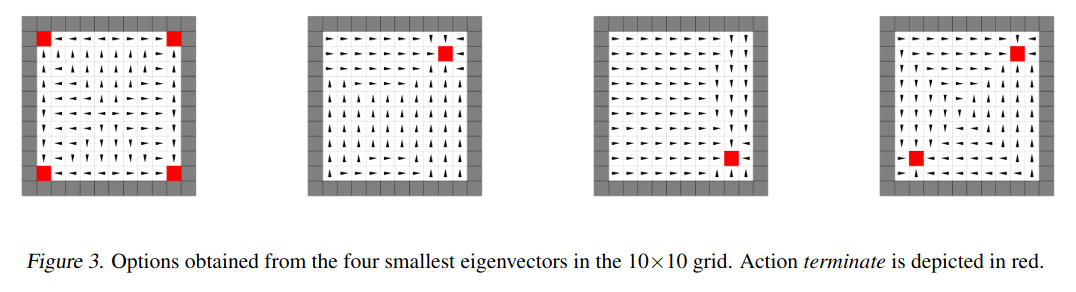
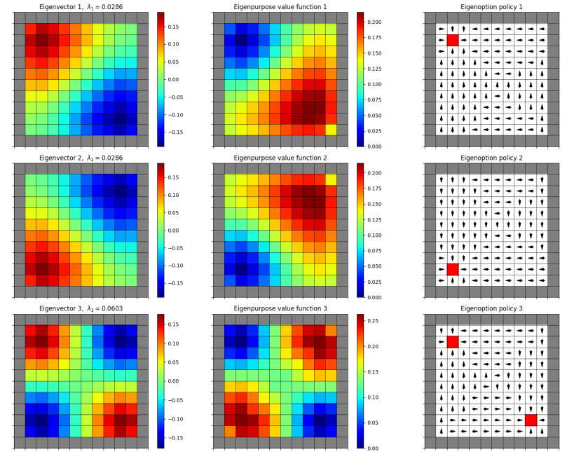
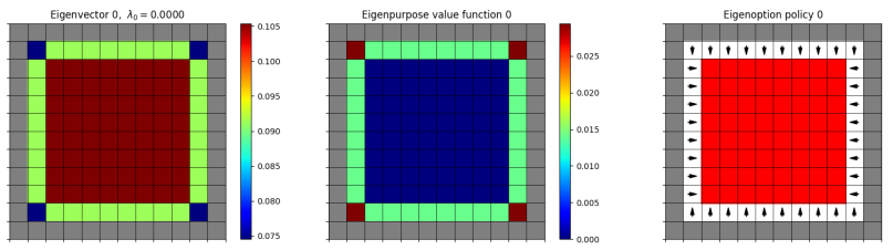
First, the simple $10 \times 10$ square grid. Theirs:
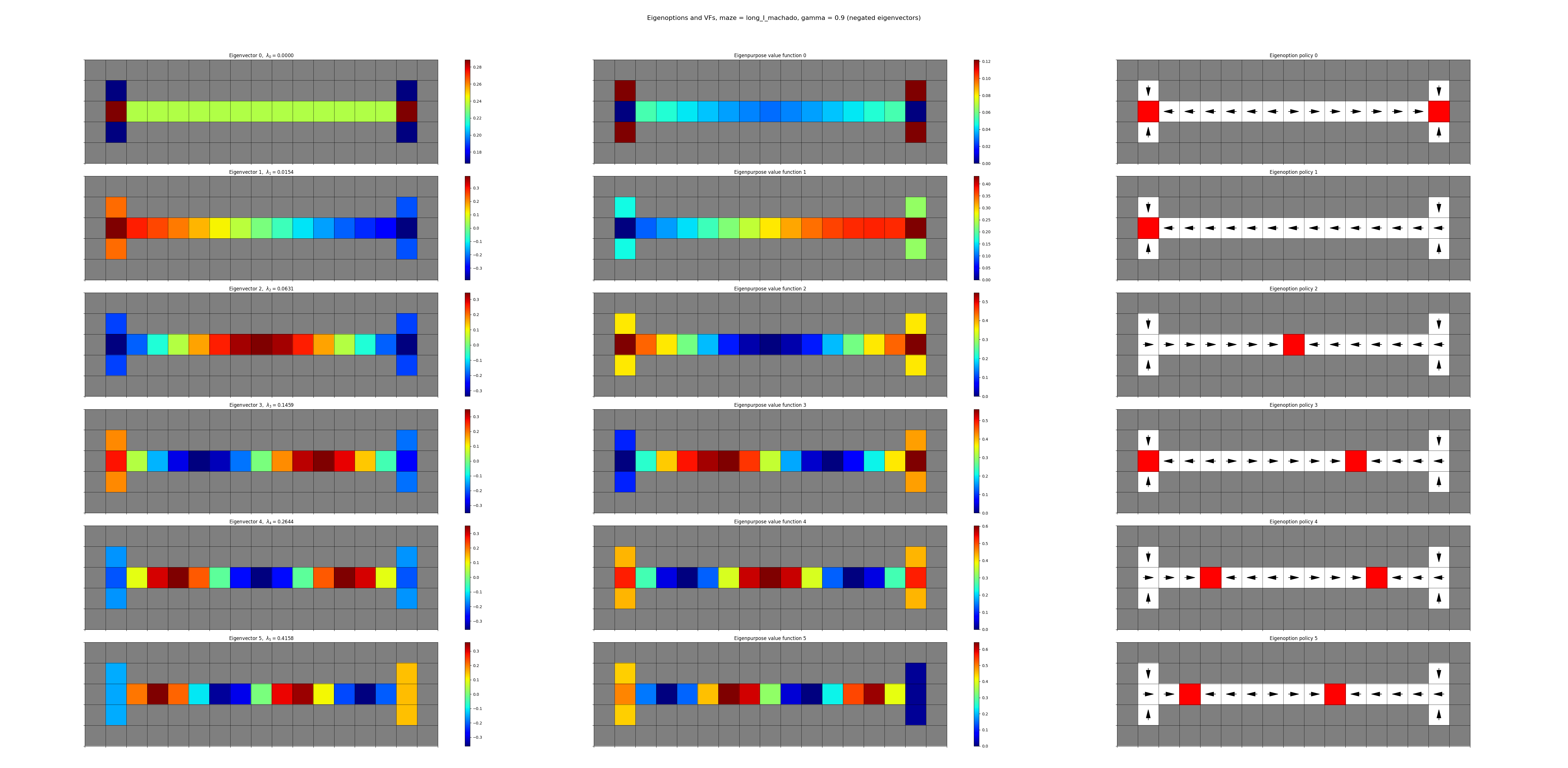
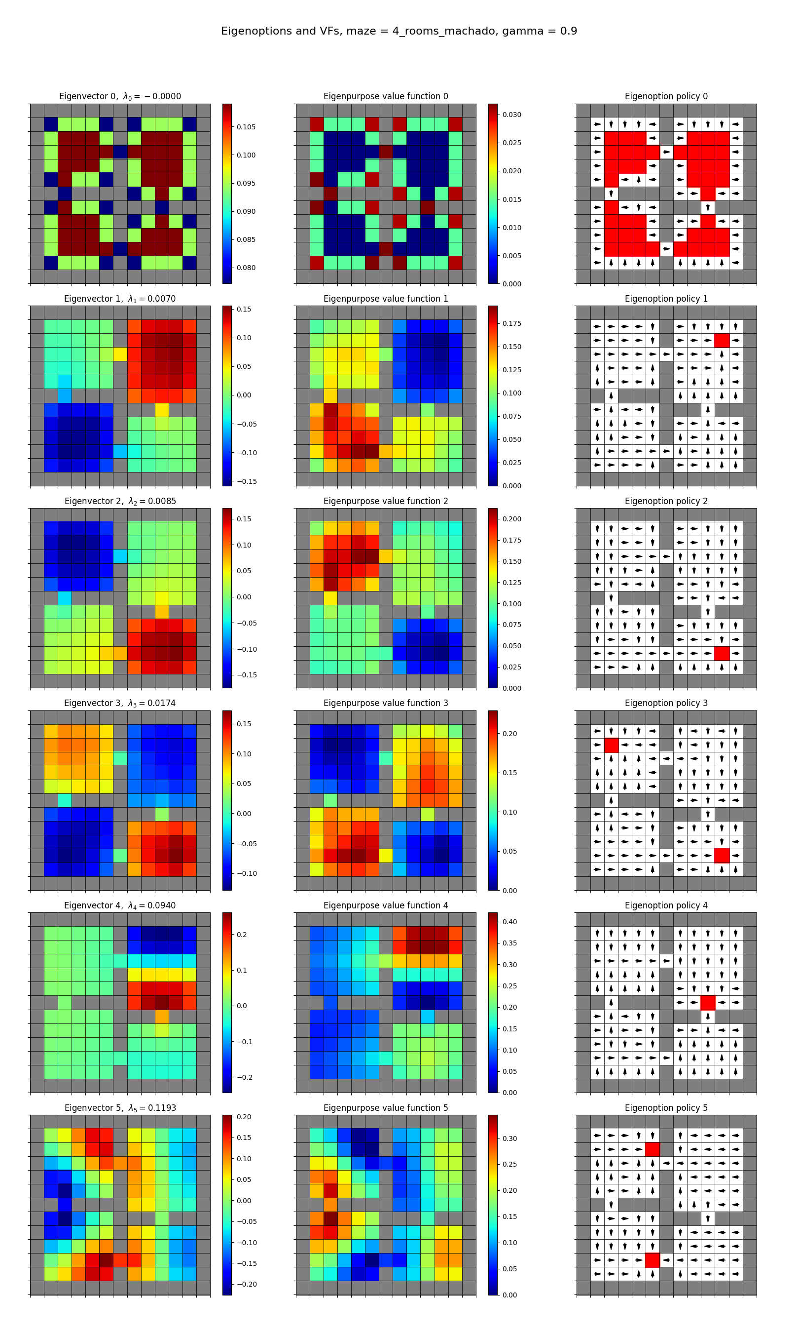
and mine:
![]()
A few notes:
- they’re showing the first four eigen-whatevers, I’m showing the first six
- the left column shows the eigenvector that gives rise to the reward function/eigenpurpose
- the middle column shows the resulting optimal VF given that reward
- the right column shows the optimal policy for that reward, with the terminal states in red
Also note that I can’t easily plot the reward itself, because it’s a function of pre- and post-action states, $r^e(s, s’) = e^\intercal (\phi(s’) - \phi(s))$, not just a single state. But you can picture it in your mind for any pair of states $(s, s’)$ by looking at the value (of the eigenvector, 1st column) of $s$ and subtracting it from the value of $s’$; it basically gets a positive reward when it’s climbing that gradient, and negative if it goes “downhill”.
This is actually an important detail. The form of the reward here, $r^e(s, s’) = e^\intercal (\phi(s’) - \phi(s))$, is nearly exactly what’s called a “potential based shaping reward”, which is one defined by a… potential function $\phi$, and generically has the form $r(s, s’) = \gamma \phi(s’) - \phi(s)$ (note that the eigenoption paper version doesn’t discount the next step from what I can see). The canonical paper that explored (/invented?) it is this Andrew Ng and Stuart Russell paper. The big takeaway is that you can add a potential based reward to any original reward function you have, and the optimal policy will remain the same.
The difference is that it might be a lot easier to the one with the potential based reward added, because it’s a much denser reward signal (as they mention in the eigenoptions paper). For example, we could’ve defined the reward for the eigenoptions above as simply zero every step until it reaches one of the maxima of the eigenfunction (i.e., a terminal state). This would give the same exact eigeoptions, but would be harder to learn since the agent wouldn’t get any reward until it discovered the goal for the first time.
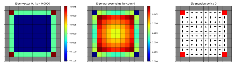
Another thing to notice about the plots is that the optimal VFs (middle column) are essentially the eigenfunctions upside-down in terms of shape, and the terminal states are located at the minima of the optimal VFs. This makes sense: when it’s far from the terminal state, it can collect a bunch of reward in the coming steps. When it’s closer to it, there aren’t many steps left to collect reward during.
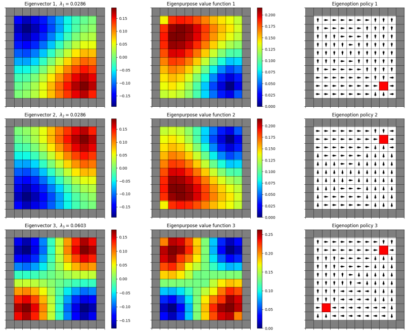
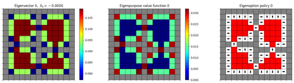
You may have noticed that some my eigenoption plots look different than his. For example, his first one has the terminal states only at the corners, while mine has it at all the squares beside the edge squares. This puzzled me at first, but then I remembered that of course the negative of an eigenfunction is also a valid eigenfunction! So I ran all the mazes for the set of eigenfunctions numpy gave, and then also for their negation (so I’ll post both going forward). That gave:
![]()
and now you can see their first one there.
Another neat thing to notice is that sometimes there are multiple terminal states, because I’m using $\gamma < 1$ discounting, and they’re the local minima of the VF. But if you look at the eigenoptions for the ones with multiple terminal states, it has the effect of partitioning the space into different regions, where the optimal behavior is to go for one terminal state versus another.
Anyway, here are the others.
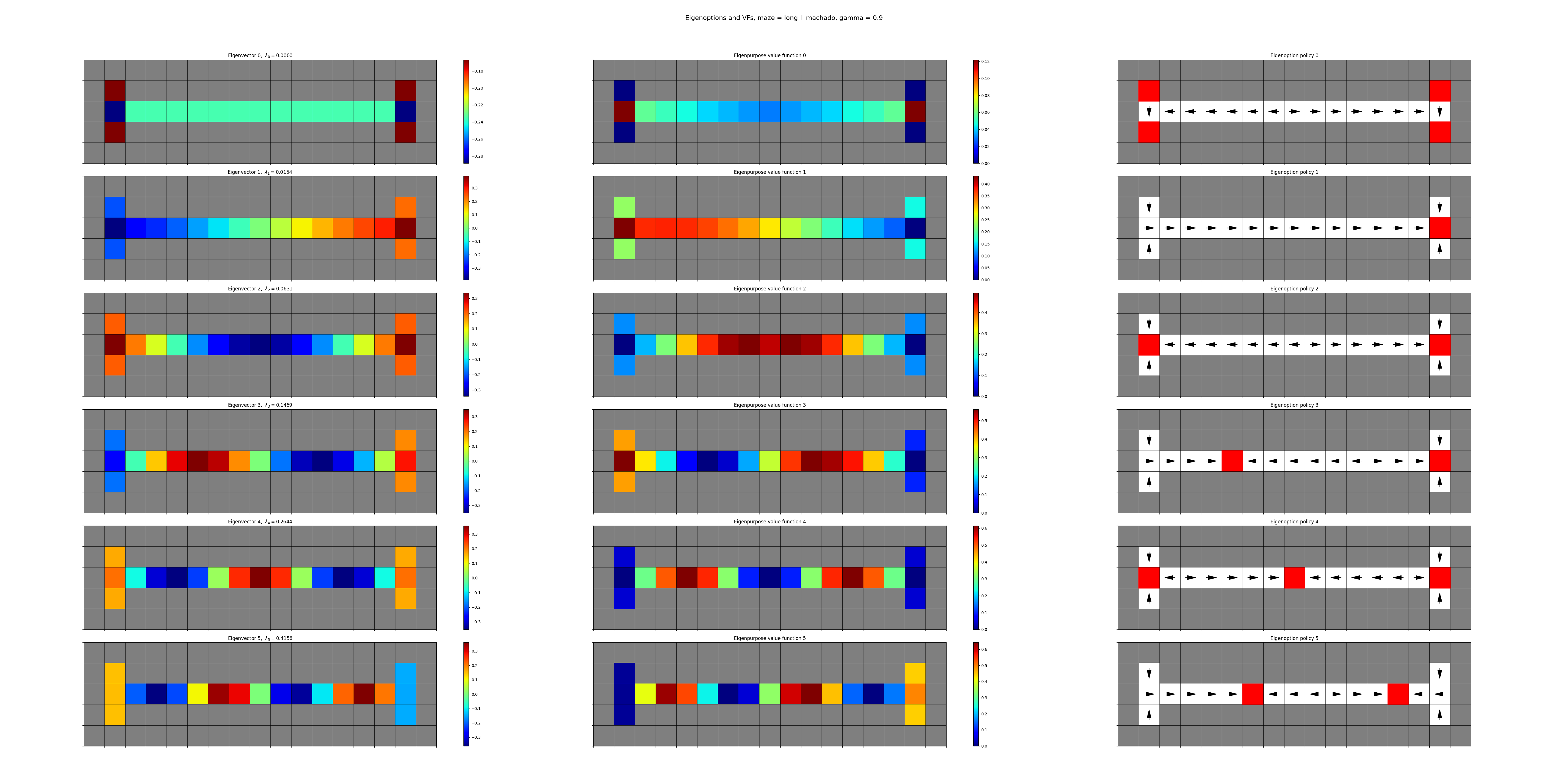
Their I-maze:
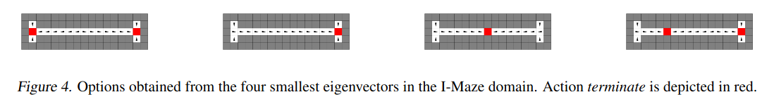
and mine, negated and not:
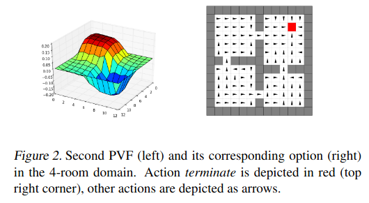
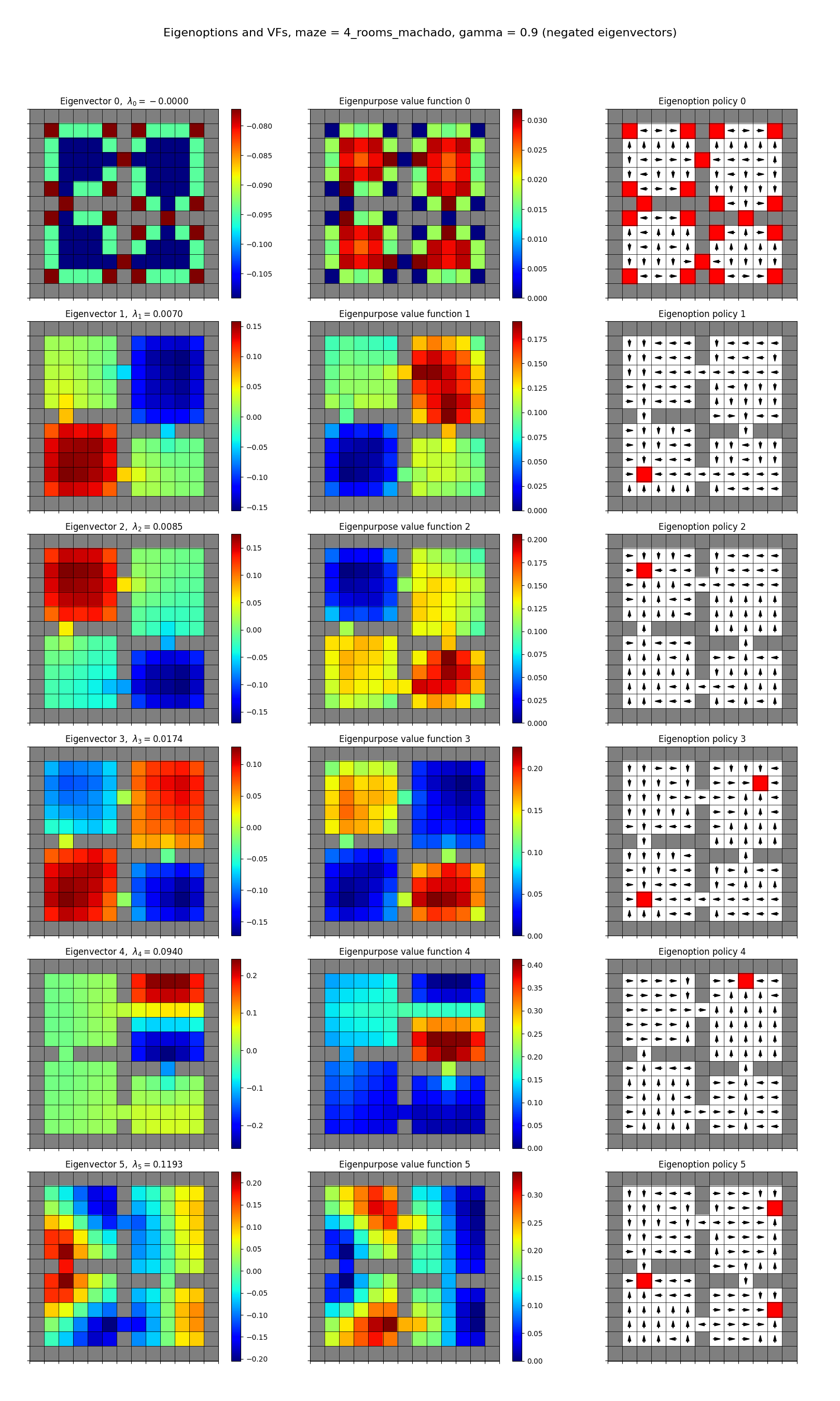
their 4-room maze:
and mine, both:
Eigenfunctions from transitions
Above, I was calculating the eigenfunctions by applying np.linalg.eigh to the adjacency matrix $A$. We’re able to get the full, true $A$ because it’s small enough and I can just iterate through all the cells and add $A_{ij}$ entries for each of the connections between adjacent cells.
However, this isn’t really possible for large or continuous state spaces; the size of each dimension of $A$ is the number of states. For their next trick, they show how you can approximate the eigenfunctions of the Laplacian without having to construct $A$.
I’m not totally sure which parts of this are original to this paper, but it’s neat nonetheless. Here’s the idea:
In addition to constructing the Laplacian as $L = D - A$, you can also construct it with the incidence matrix $T$, as $L = \frac{1}{2} T^\intercal T$. This much isn’t new; it’s on Wikipedia. However, on wiki, it’s still assumed that you have the “full” $T$ in the same way you technically need the “full” $A$. They show that you can approximate $T$ with samples. To do this, for each transition $(s, s’)$, we add $(\phi(s’) - \phi(s))$ as a row to $T$.
What seems like the real insight here is that with this $T$, we can calculate the SVD for it, $T = U \Sigma V^\intercal$. Then, because $L = \frac{1}{2} T^\intercal T$, the columns of $V$ will approximate the eigenvectors of $L$. In the case where $\phi(s)$ is a one-hot vector and we managed to sample every transition at least once, the columns of $V$ will be exactly the eigenvectors. Again, this is basic linear algebra, but it does seem like a clever connection to make.
(by the way, I think there’s a minor error here in their theorem 5.1 – the last sentence should say “the orthonormal eigenvectors of $L$ are the rows of $V^\intercal$”.)
I don’t have much to show here. I made it calculate the incidence matrix with a one-hot rep and all transitions, and did SVD with it, and verified that the eigenvectors are exactly the same (up to sign), the eigenvalues are the same as the singular values squared and divided by two, and the matrices are exactly the same. But it’s not exactly thrilling to show a bunch of print statements asserting that one thing minus the other equals zero, so I’ll skip that.
In the paper, they use the Atari emulator’s RAM state as the representation $\phi$, which I thought was neat. It’s $1,024$ bits and my impression is that since it’s RAM, it’s not going to be directly “meaningful” if you or I looked at it. But it’s a good illustration of the method, since the $T$ they construct with it (using 25k transitions) lets them calculate some useful eigenfunction approximations!
I’ll actually be doing this in a near-future post on another paper where they compare to this one, so I’ll save that implementation and results for then.
Errata
The options for negative eigenfunctions are sometimes very different?
I thought this was curious (it’s also possible I made a mistake here). If you compare the eigenoptions for versions where I did vs didn’t negate the eigenfunction before calculating the optimal VF/policy, most of them are pretty similar, just switching a location of a terminal state (and the resulting direction of the policy). For example, negated and original:
Negated:
Original:
However, comparing the first eigenfunctions, negated:
original:
They’re clearly way more different; one seems to be kind of an “inverse” of the other. The “original” one would terminate after one or two steps, whereas the negated one has more going on. This is the same for the other mazes too, for example:
original:
negated:
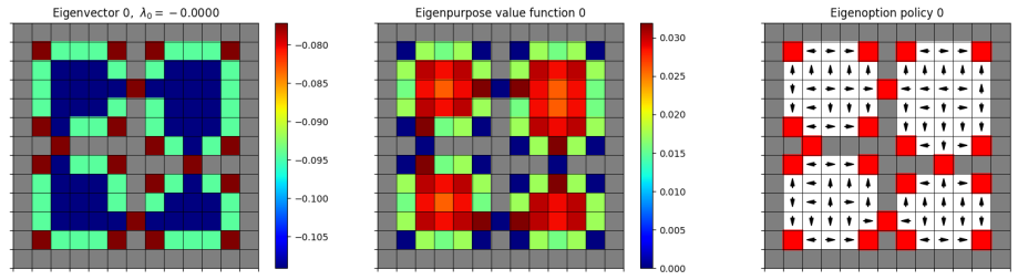
I doubt this is a bit deal, since the other eigenoptions seem to be more similar regardless of the eigenfunction sign, and you’d typically use a bunch of them for an application. But, the fundamental one is also pretty important usually. So I’m not sure what the significance of this is, or whether it really matters. I suppose you could try and figure out which version has fewer terminal states, and use that one (since they seem to be more interesting).
Discounting
Remember that above I said that the eigenoption termination states are meant to be for when it has “achieved its eigenpurpose”, meaning that the agent’s in a state where it can’t collect any more cumulative rewards. Let me quote them ($\chi^e$ is the eigenbehavior/policy for eigenpurpose $r^e$):
When defining the MDP to learn the option, we augmented the agent’s action set with the terminate action, allowing the agent to interrupt the option anytime. We want options to terminate when the agent achieves its purpose, i.e., when it is unable to accumulate further positive intrinsic rewards. With the defined reward function, this happens when the agent reaches the state with largest value in the eigenpurpose (or a local maximum when $\gamma < 1$). Any subsequent reward will be negative.
We are able to formalize this condition by defining $q_\chi(s, \perp) = 0$ for all $\chi^e$. When the terminate action is selected, control is returned to the higher level policy. An option following a policy $\chi^e$ terminates when $q^e_\chi(s, a) \leq 0$ for all $a \in \mathcal A$. …
I’m… a little confused here, if I’m honest – they say that termination should happen when the agent can’t accumulate more rewards, which “happens when the agent reaches the state with largest value in the eigenpurpose”. I think it should be smallest value, right? It has the largest value when it’s farthest from the termination state, unless I’m missing something.
Anyway, the more interesting piece in that quote is about the effect of discounting. Here’s the 4-rooms plot (not negated) from earlier, but with $\gamma = 0.999$:
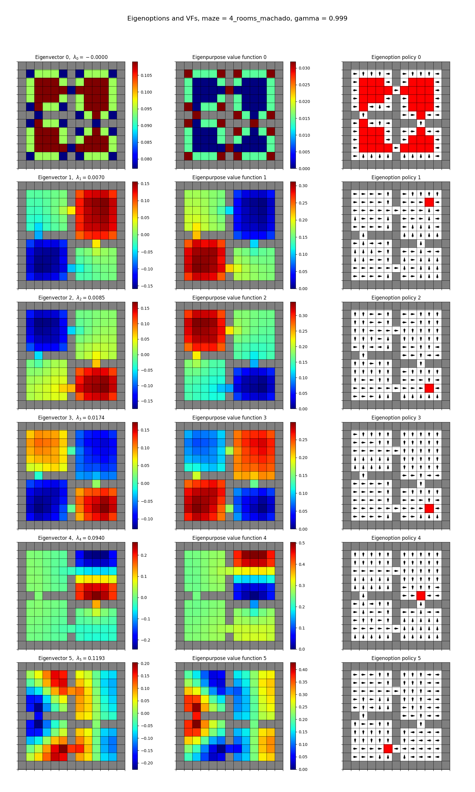 and next to the earlier $\gamma = 0.9$ one, for your viewing pleasure:

Notice anything? In the cases where there were previously two terminal states, there are now one. Why?
In their quote they said “With the defined reward function, this happens when the agent reaches the state with largest value in the eigenpurpose (or a local maximum when $\gamma < 1$). Any subsequent reward will be negative.”
You can see that in the cases where there were two terminal states for $\gamma = 0.9$, they line up with the minima of the VF, and when $\gamma = 0.999$, the only one is at the global minima like they say. This happens because in both cases, if the agent is at the the local-but-not-global minima, the rewards in the next few steps will definitely be negative (i.e., it’s at an eigenfunction local maximum and going downhill). However, if the agent kept going through this valley, it’d eventually lead to a path to the other, global minima, where the rewards collected would be greater than what it lost.
However, this is where discounting has its effect. For $\gamma = 1$, you can write the sum of rewards over steps from the local to global minima, ${s_1, s_2, \dots, s_{k+1}}$, as:
\[\begin{aligned} \sum_{i=1}^k r^e(s_i, s_{i+1}) &= \sum_{i=1}^k e^\intercal (\phi(s_{i+1}) - \phi(s_i)) \\ &= e^\intercal \bigg[ (\phi(s_{2}) - \phi(s_1)) + (\phi(s_{3}) - \phi(s_2)) + \dots + (\phi(s_{k+1}) - \phi(s_k)) \bigg] \\ &= e^\intercal (\phi(s_{k+1}) - \phi(s_1)) \\ \end{aligned}\]So you can see that all the terms except the first and last cancel out! This is basically a property of potential based rewards. So this means that when $\gamma \approx 1$, it’s always worth it for the agent to go to the global minima, because it’ll net positive cumulative reward.
On the other hand, with $\gamma < 1$, the above becomes:
\[\begin{aligned} \sum_{i=1}^k \gamma^{i - 1} r^e(s_i, s_{i+1}) &= \sum_{i=1}^k \gamma^{i - 1} e^\intercal (\phi(s_{i+1}) - \phi(s_i)) \\ &= e^\intercal \bigg[ (\phi(s_{2}) - \phi(s_1)) + \gamma (\phi(s_{3}) - \phi(s_2)) + \dots + \gamma^{k - 1} (\phi(s_{k+1}) - \phi(s_k)) \bigg] \\ \end{aligned}\]and this doesn’t have the nice cancellation effect that it did before. But you can see that the effect is that it’s weighing the future rewards less (…obviously, that’s kind of the meaning of $\gamma < 1$), meaning that for some $\gamma$ value, it becomes not worth it to go through the “valley”.
Combinatorial vs normalized Laplacian?
This is one aspect of this paper that could’ve been made a bit clearer. At the beginning when they’re presenting the Laplacian, they say:
PVFs are defined to be the eigenvectors obtained after the eigendecomposition of $L$. Different diffusion models can be used to generate PVFs, such as the normalized graph Laplacian $L = D^{-1/2} (D − A)D^{-1/2}$, which we use in this paper.
The normalized Laplacian is another one of several versions of the Laplacian that people use, because it has some nice properties. However, it is different than the “combinatorial” Laplacian (i.e., $L = D - A$); its eigenvalues are the same but its eigenvectors are different.
What’s kind of confusing here is that they say they use the normalized GL, but their theorem 5.1 is definitely concerning the combinatorial Laplacian. They’re not super clear on when they’re using one Laplacian versus the other, or any significance of doing so. My best guess is that they use the normalized GL for the mazes, where they can just calculate whatever anyway, and use the Theorem 5.1 version for their Atari experiments, and that one will approximate the eigenvectors of the combinatorial Laplacian.
That said, it’s unclear to me how much it matters. It seems like the motivation for them in the first place is a somewhat handwavy “they represent fundamental structure of the env” and it doesn’t matter so much exactly what they are.
Neato. I learned a lot! Many giggles were had and many plots were made. See ya next time!