Rotational invariance strikes again! Proto VFs and proto RL
I’ve been going ham on the Laplacian recently! 🍖 Ham 1, ham 2, ham 3. It’s definitely interesting for its own sake, but I was initially motivated by a few RL papers that used it, and now we’re finally here. The papers that got me looking into it are more recent (~2018), but most of them have their background in a much older one that I’m looking at today and implementing some of.
The paper in question is “Proto-value functions: developmental reinforcement learning” (2005, ICML, alternate link with PDF). It’s… a strange bird, if I’m honest. It’s a measly 8 pages including many figures, but they spend quite a lot of the text talking about the more advanced math that the ideas in the paper have connections to… but don’t actually really use any of it?
Anyway, it’s still a cool paper and is the one pretty much all Laplacian RL papers have to mention. Let’s get into it.
Motivation
The main motivation for the paper is representation learning for RL. I.e., finding a representation that we can express the value function (VF) in, that will make learning easier, and be task independent. The high level idea can be summed up like this:
- the state space and transition matrix of an RL env can be viewed as a graph
- since it’s a graph, we can look at the Laplacian of it
- we know that the eigenfunctions of the Laplacian represent some interesting fundamental aspects of the graph
- if we can find these eigenfunctions, we can use them for lots of things
- the Laplacian relates to the dynamics of the env, and is unrelated to the reward (i.e., task), so it can be helpful for any task
These eigenfunctions will be viewed as possible VFs, ${V_i}$, and specifically they’ll be viewed as basis functions we can use to construct any other function. For example, usually we want to learn $V^\pi$, the VF for policy $\pi$. But if the $V_i$ form a complete basis, then we can express $V^\pi$ as a linear combo of them:
\[V^\pi = \sum_i \alpha_i V_i\]Since there are usually many states, if we could express $V^\pi$ with a relatively small number of $V_i$ components, it might make it easier to just learn the necessary $\alpha_i$ weights than learn a whole VF.
To sound cooler, they call them “proto VFs” (PVFs). But there are many possible complete sets of basis functions we could use… Why do we want to use eigenfunctions of the Laplacian for them?
What makes them really useful is that they reflect the graph topology and the structure inherent in the dynamics in a way other ones might not. As a simple example, let’s say our env is this maze:
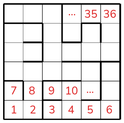
and the states are represented as increasing integers like in the pic. If we tried using, say, a Fourier basis in terms of that state representation, it’d… well, it’d give us something. But it probably wouldn’t be very useful, because those number labels are mostly not related to each other in a very meaningful way. For example, a Fourier component $f$ (let’s say a sine) is locally fairly smooth in its arguments. However, in the maze above, states 2 and 8 are next to each other, but $f(2)$ is likely very different than $f(8)$.
Okay, you say, but I chose a really weird choice of labeling the states. No one would do it like that. Isn’t it much nicer to do it with some 2D coordinates, like this?
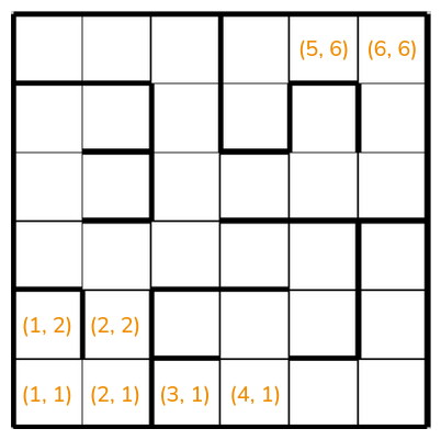
Now, the trouble cells from before are $(2, 1)$ and $(2, 2)$, and if we used a 2D Fourier basis of it, it’s pretty likely that $f(2, 1) \approx f(2, 2)$ like we wanted. Problem solved!?


NOT SO FAST BUCKO
We still have a problem: $(2, 1)$ and $(3, 1)$ are next to each other and will therefore have $f(2, 1) \approx f(3, 1)$, but… they shouldn’t! It’d take a minimum of 9 steps to get from $(2, 1)$ to $(3, 1)$. Even if they’re next to each other in the grid, they’re not close to each other in the sense you probably care about if you’re in a maze.
Basically, we want a representation that learns about the “meaningful” structure in the env, not just some naive structure that’s a result of whatever representation we happen to be using. You might say that we should just choose a representation that makes more sense in the first place, but more generally we shouldn’t be expecting to choose a representation, or get one that’s straightforward, and instead be making methods that can learn from any one, as long as the info is there in some form. And that’s what we’ll use the Laplacian for, because it’ll try to capture the meaningful structure.
Real Gs might find all this talk about “meaningful structure” reminiscent of my posts on distances in pixel space and thin manifolds. That’s because it’s basically the same idea again, just a different method for attacking it.
Making the magic happen
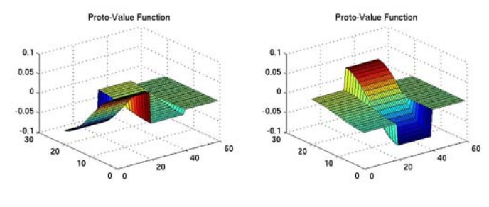
Alright, so let’s give it a whirl. I’m gonna try implementing it to try and reproduce the figures in the paper. Here’s Fig 1:
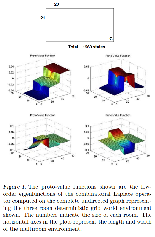 The env here is that 3 room maze, where each room has $21 \times 20$ cells, and there are those three rooms separated by small doors, for a total of $1260$ states. That means that the “graph” of this environment has $1260$ vertices, and the edges between vertices are defined by whether the agent can go from from to the other in a step. The edges between the vertices effectively define the whole problem, since they specify the adjacency matrix $A$.
You could calculate $A$ based on just observing transitions, but here I’m just going to construct it directly by iterating through all the maze cells, and for each one, looking at its immediate (U, D, L, R) neighbors, and adding an edge in $A$ for each.
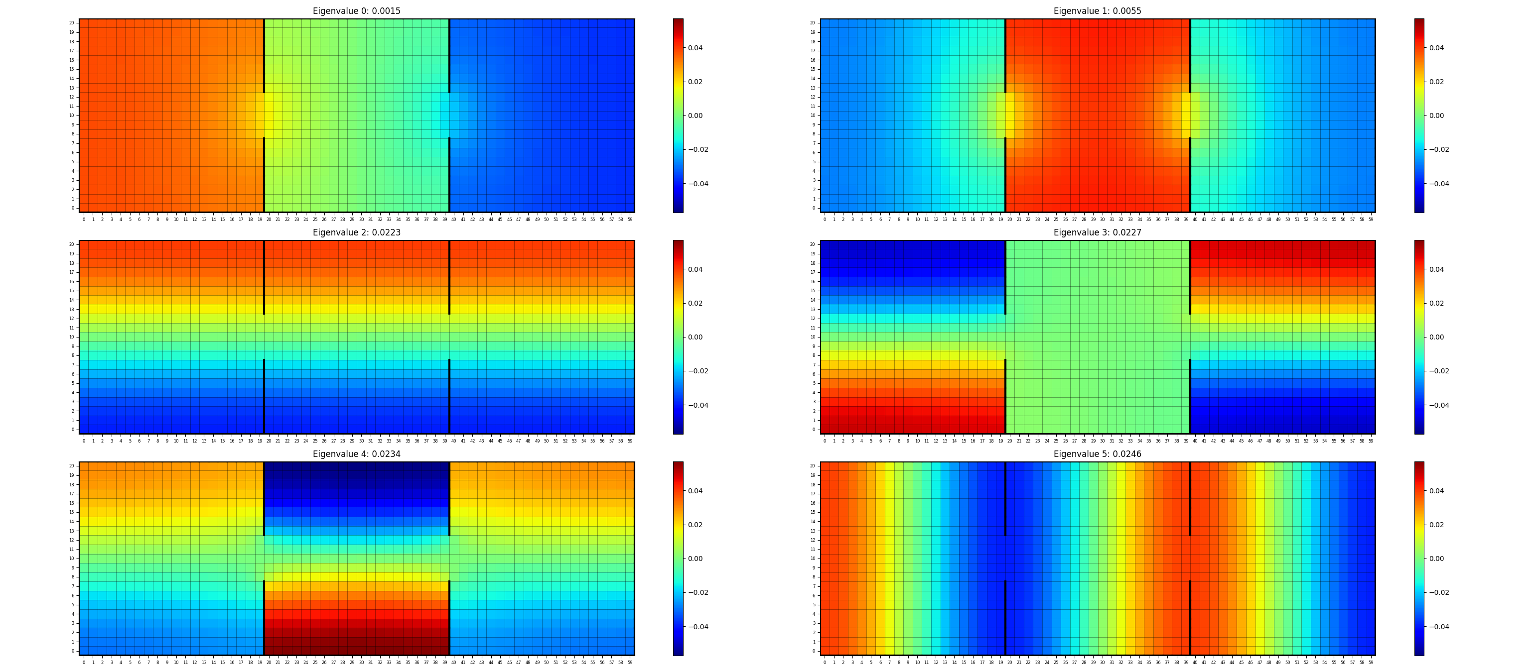
Once we have $A$, we have $D$ and can calculate $L = D - A$. And again, the number of states is small enough that I can just hammer it with a np.linalg.eigh to get the eigenvalues and eigenvectors.
That gives us (the first 6, skipping the constant eigenfunction):
and in 3D, like theirs:
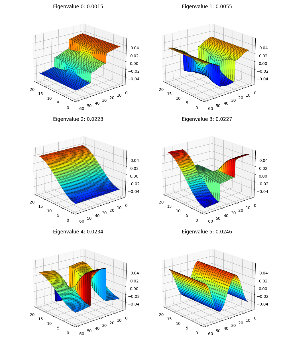
Not bad! But… if you look close, something’s definitely a bit off. You can see that my upper left one is their UL one, and my UR one is their UR one, but their two on the lower row aren’t here… Hmmm. Maybe they’re just a bit out of order? Here are the first 15 to be sure:
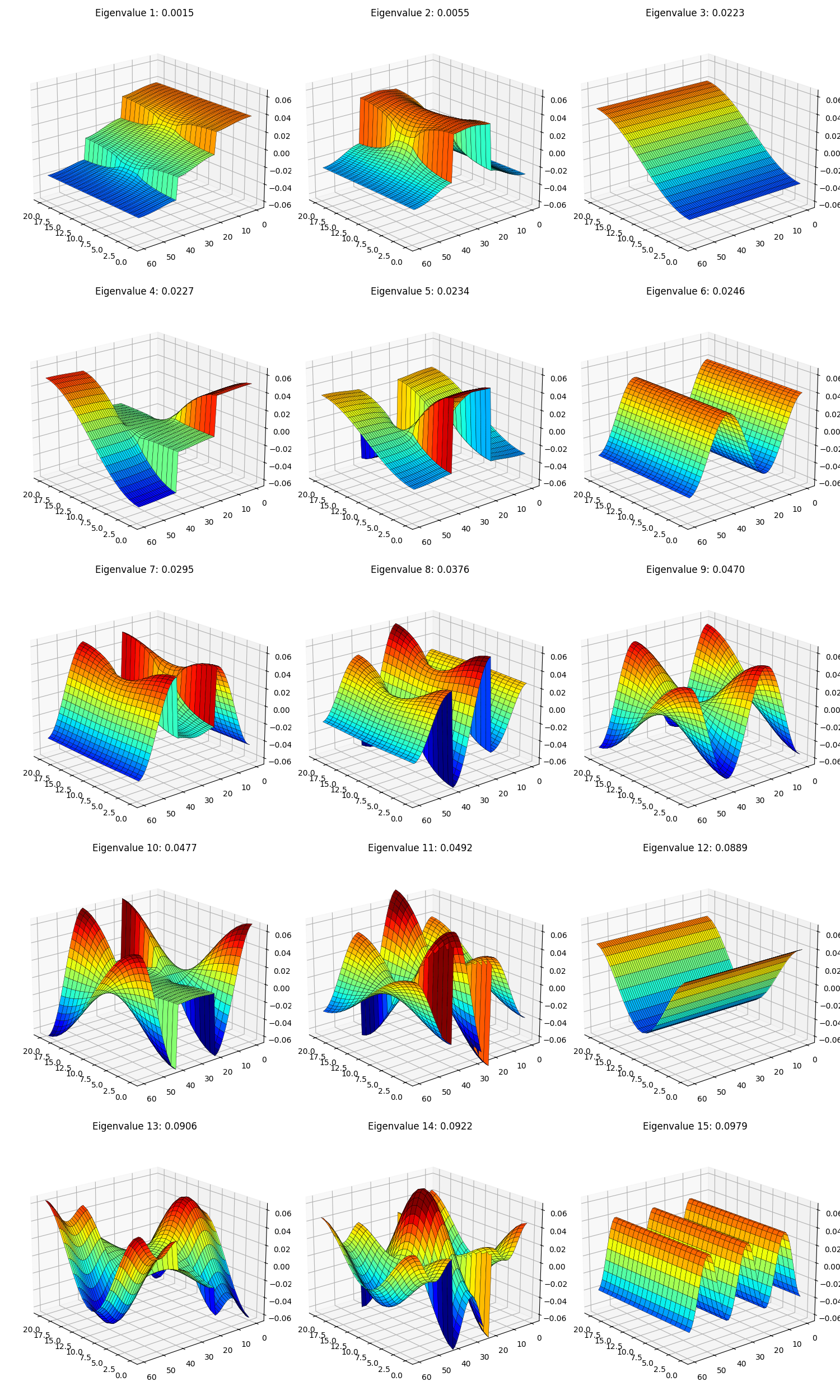
Very pretty, but they’re still not there… Any guesses?
Rotational invariance inside a subspace strikes again! One clue is that if you look at the eigenvalues in the axis titles, the 3rd, 4th, and 5th ones eigenvalues are all in the range $0.223 - 0.234$, implying that that eigenvalue has some multiplicity and multiple eigenfunctions associated with it.
When I was trying to optimize the eigenfunctions with gradient descent, I painfully discovered that the optimization yielded a set of orthogonal functions that minimized the energy objective, but weren’t actually the eigenfunctions themselves, just an orthogonal rotation of them. This case is slightly different, but a similar idea. It’s different because in the previous case, the functions actually had different energies, but their sum was equal to the true eigenvalues’ sum. In this case, they actually all have the same eigenvalues/energies, there are just multiple ones that share that eigenvalue. Therefore, it’s not really a matter of an optimization procedure not finding the specific solution we want, there actually isn’t a specific set of eigenfunctions for this eigenvalue that are the “true” ones. The “true” eigenfunctions for $\lambda \approx 0.225$ are any three orthogonal ones in that subspace.
But enough of the gobbledygook. Speak english, doc! We ain’t scientists.. How do we make pretty picture B look like pretty picture A??
I’m gonna be honest, there are smarter things you can do. But I basically squinted and it sure looked like theirs looked like pretty simple linear combos of the ones in my plots, so I just tried a few combos by hand until they looked pretty similar, and ended up with these to match his bottom row:
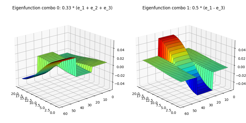 Eh? Eh??
 Close enough for bluegrass, as they say. Perfect is the enemy of the good, they say.
The other thing I wanted to try from the paper was building a given VF from a basis of these Laplacian basis functions, i.e., $V = \sum_i \alpha_i V_i$. They have an example of that in their Fig 2:
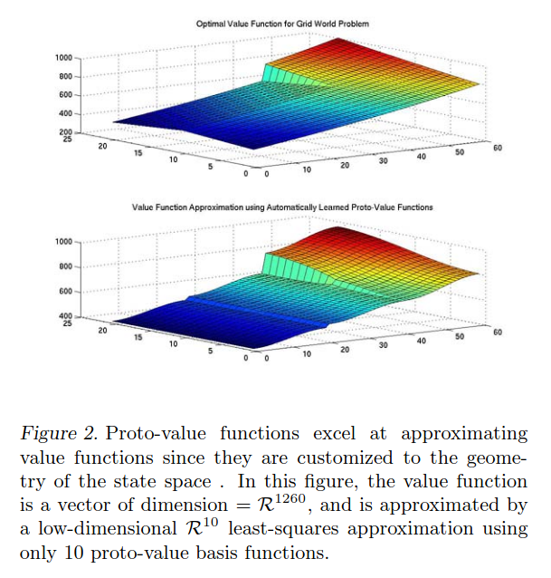
The VF they’re trying to build is the optimal one for the goal position shown in their Fig 1 (flipped upside down I guess). You can see in the top plot there that the VF rises as it gets closer to the back corner where the goal is, but that there’s also a fairly sharp “cliff” where the VF changes sharply between adjacent cells because of the wall (i.e., they’re adjacent in terms of cell coordinates but not steps, like we saw above). I just calculate $V^\ast$ using value iteration, which is easy because it’s just tabular and we know the neighbors of each state.
Since the Laplacian eigenfunctions $V_i$ are orthonormal to each other, it’s easy to calculate the $\alpha_i$ coefficients. We assume $V^\ast = \sum_i \alpha_i V_i$, and then
\[\langle V_i, V^\ast \rangle = \langle V_i, \sum_j \alpha_j V_j \rangle = \sum_j \alpha_j \langle V_i, V_j \rangle = \alpha_i\]You can choose to use as many components as you want, and of course the more you use the closer it’ll be to the real function. They use 10, so that’s what I use here:
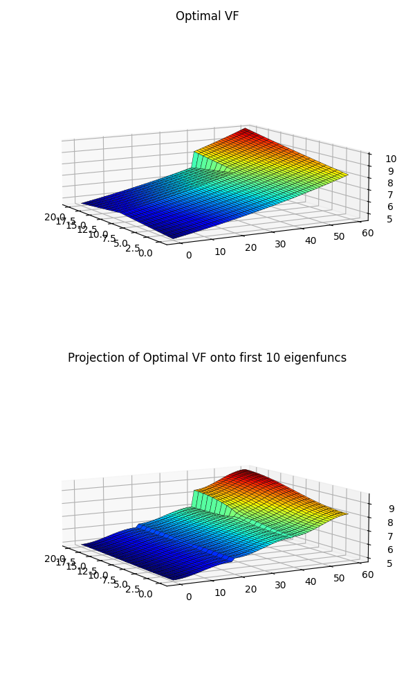 Hot DAYUM that looks pretty similar to theirs. You can see that for both of ours, the projected version has a little “curvature” leading away from the cliff that the true VF doesn’t.
We can also look in 2D, and plot their difference to see where the errors are largest:
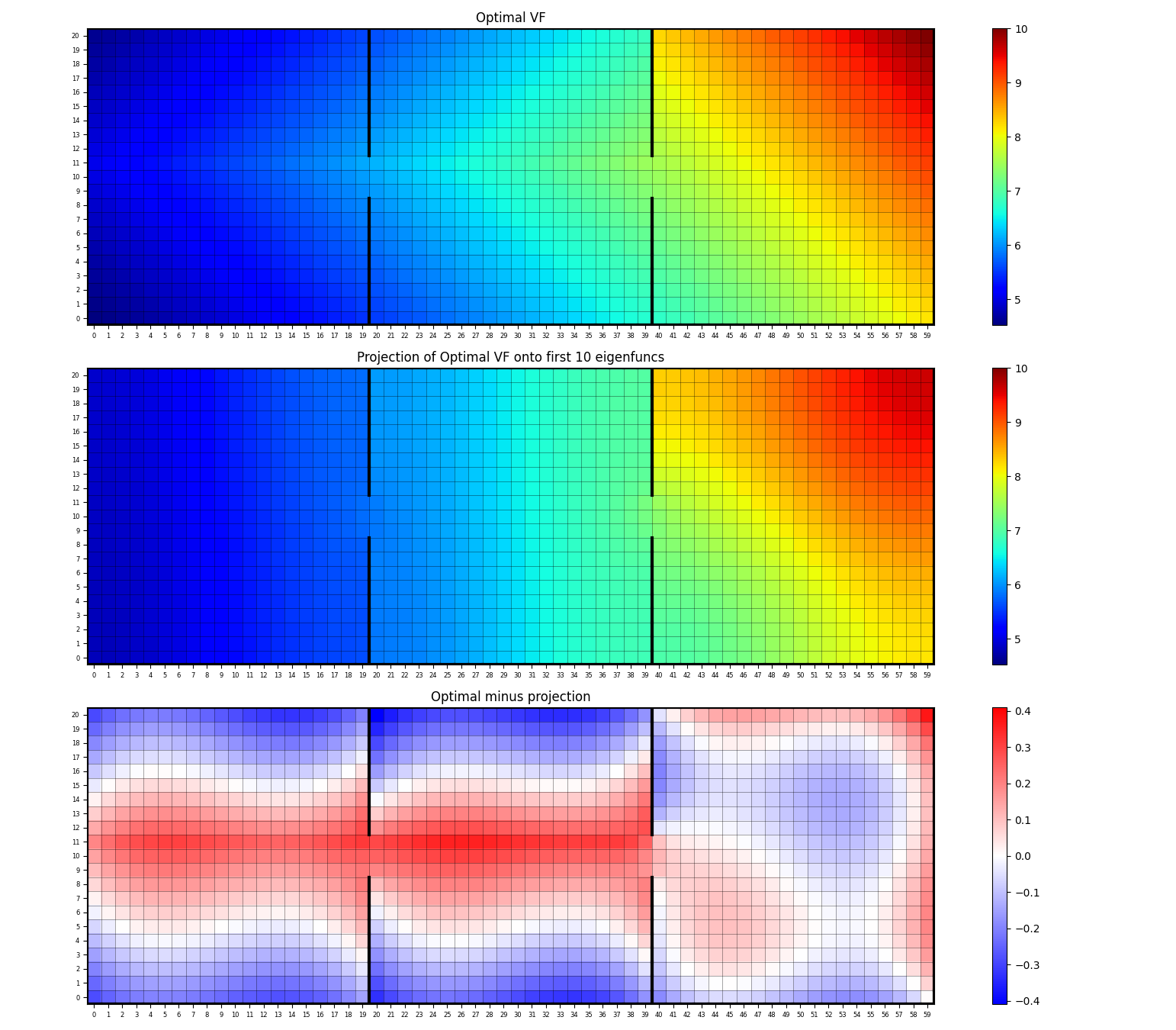
It looks like the main thing it has trouble approximating with these first 10 are the “diagonal” shapes of the VF in the 1st and 2nd rooms. I dunno.
Lastly, it’s a reasonable question how quickly the error would drop if we used more components. That’s what they have the next two figures for:
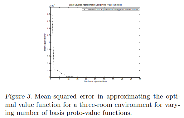
Figure 3 is basically just doing what I did above, but for increasing numbers of components. Here’s what I got:
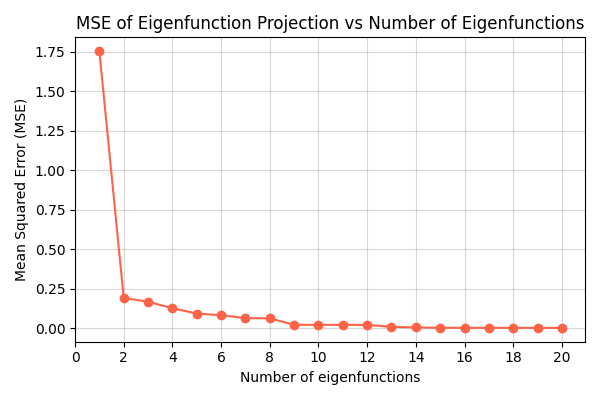 Close enough?
And they have this one:
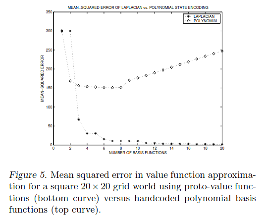 Note that Fig 5 is for a different grid world. It might seem strange that the polynomial basis functions they compare to start increasing their error with more basis functions – shouldn’t it only be better, and you can just choose not to use them if they’re unhelpful? The answer is that for this plot they’re fitting the basis coefficients based on the target VF only being defined at some states, not all states as I (and them in Fig 3) did above. This means the polynomial ones overfit to the data they do have when they have more (higher order) terms. I’m wondering if the Laplacian ones will eventually overfit, or whether something about them has some inherent regularization or something. Nothing’s for free, so I’m guessing they just start overfitting later.
Alllllllrighty, that’s enough for today. They also come up with a little control algo using this, but it’s based on LSPI and LSTD and other things I don’t want to deal with today. I think the things above are the more important takeaway anyway.
Next time I’ll look at a much more recent paper that picked up where this one left off. See ya then!