A guessing game with thin manifolds
A simple guessing game
Let’s play a little game. I’ll show you a few example pictures, and you have to give me another picture that I could’ve produced, i.e., drawn from the same distribution. Okay, here’s your first batch:
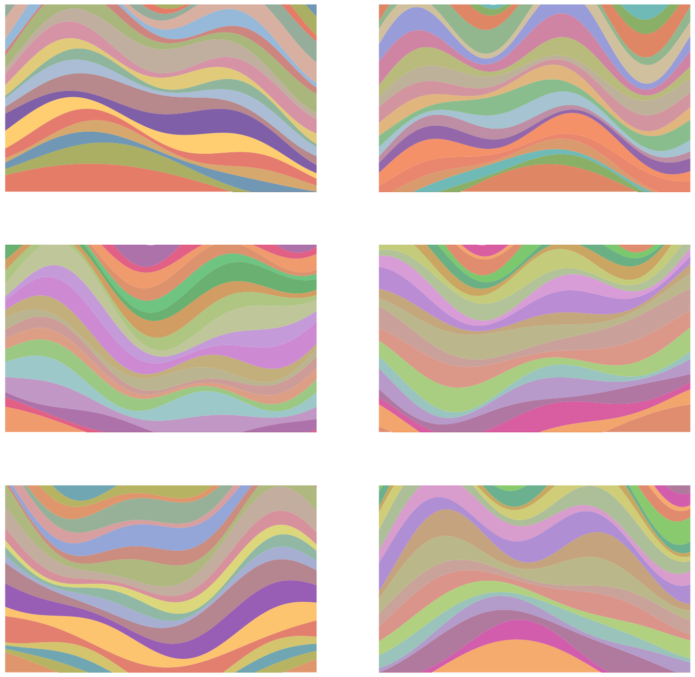
Got it yet? No? That’s alright, here are a few more:
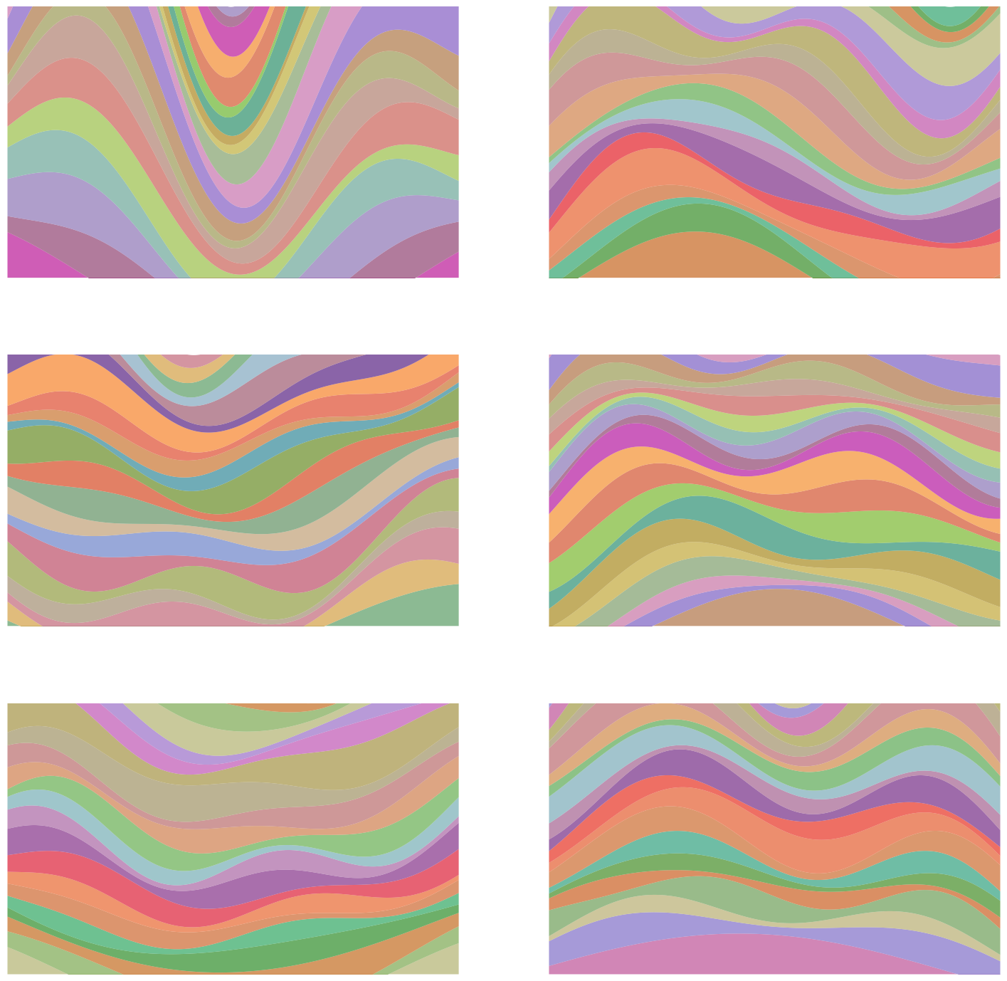
Surely you must have it by now! I mean, it’s a rather elementary 1D distribution, after all 🙄.
How about this one?
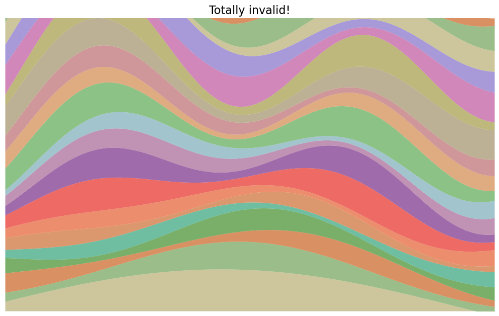
Sike! That’s not one I would’ve produced, silly.
What’s the point of this, anyway? Let’s take a step back to motivate it.
The data manifold
My true fans (hi mom) will recognize this from my old Sol Lewitt post, slightly modified. I was going to come up with another example before realizing that this was actually a perfect fun example for what I want to say.
The problem we’re solving here is this: we’re given some example data that comes from some real data distribution, and we want to produce more points like the ones from that distribution. However, the data examples are in some super high dimensional space, and it’d be pretty tricky to figure out the pattern among them so that we could produce new ones.
How high dimensional? Well, given that each pixel has an RGB value, an image has pixel dimensions of $(H, W, 3)$, so naively that’s a $H \times W \times 3$ dimensional space… pretty big!
But why does the data being in such a high dimensional space mean that it’s hard to produce other samples like it?
Let’s imagine trying to produce similar samples to the ones in our dataset by naively adding some noise to a data sample, or maybe interpolating between two samples.
The trouble is that if you took one of my examples and tried to slightly change it “locally” in some way to get another valid sample, the vast majority of changes you could make would result in an invalid example. For example, imagine adding a layer of uncorrelated Gaussian noise over the whole image, or bumping up the blue channel value of a single pixel: most of these changes wouldn’t look like a valid one of these Sol Lewitt drawings, let alone my special collection of them.
This isn’t just because it’s high dimensional, though! Recall that I mentioned above that my Sol Lewitt distribution was fundamentally a 1D distribution, and this is actually key.
To see this let’s look at some much simpler examples.
Here’s a simple 2D gaussian distribution:
If we look at the point inside the circle and imagine perturbing it a bit in any direction (i.e., the example arrows), we see that the density at the new point might change a little, but it’s still going to be in the distribution and have a fairly similar density. Importantly, this would still be the case if it were instead a 100-dimensional Gaussian distribution.
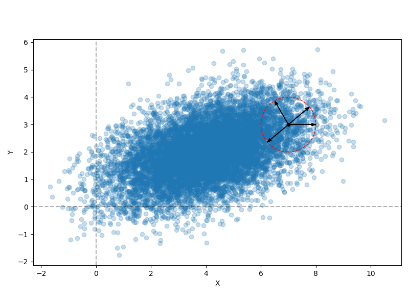
Now, I’m again generating 10,000 points from a 1D standard Gaussian $t \sim \mathcal N(0, 1)$, but applying the function $t \mapsto (x(t), y(t)) = (2t, 2t + \sin t + 0.3 \sin 5 t)$ to embed them into 2D space (the colors are just labeling the inputs $t$ from smallest to largest):
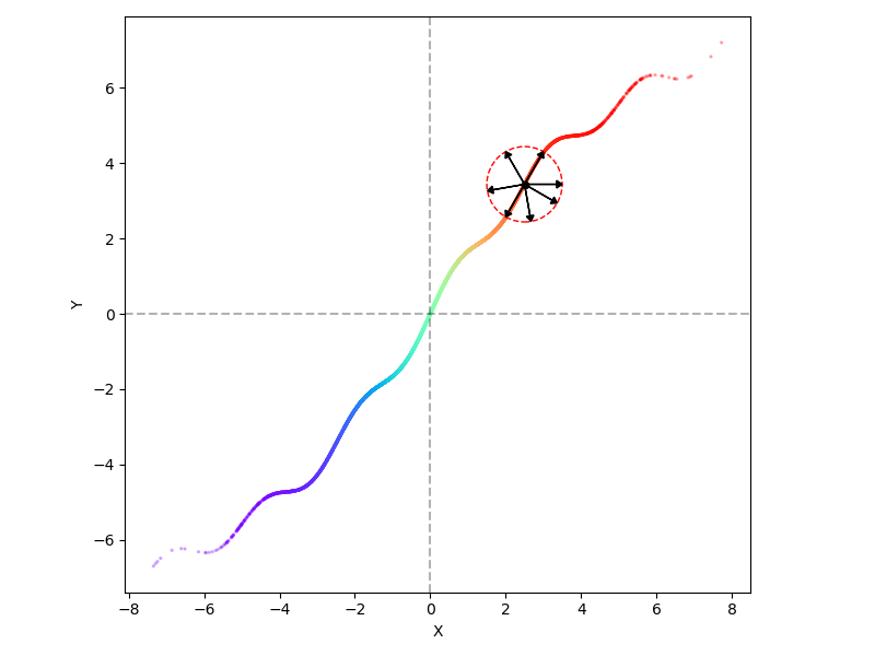
Now, if we try the same idea as before with applying a small perturbation at a given point, like the one in the center of the circle, we can see that in contrast to before, only two directions, along the tangent direction at the point, actually produce valid other samples. The majority of other perturbations produce points that are not in the distribution.
And, this is going to get worse, the bigger the space that the distribution is embedded into. Here’s the same 1D standard normal distribution, but embedded into 3D:
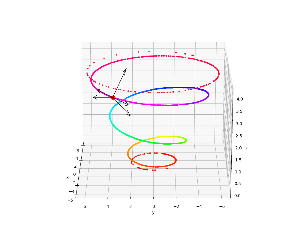
Almost all directions are now off of the data distribution!
This is basically just the famous “manifold hypothesis”, the idea that for many datasets, the data is actually a lot lower dimensional than the space it’s presented to us in. I.e., old news.
But in my opinion we shouldn’t even call it a “hypothesis”, because it’s just true, for most real datasets! For example, even for a dataset that’s a very diverse set of images, there are tons and tons of things you just would never expect to see, both in terms of higher level content, but also pixel level features like I mentioned above (for example, having a random block of a single color in part of the image).
So what can we do?
There are kind of two problems if we want to be able to be able to produce samples that resemble the true distribution, that are related but not exactly the same:
- In the original (higher dimensional) space, the data doesn’t “fill the space” because it’s inherently lower dimensional
- Even if the data did fill the space, it might have a strange density that’s difficult to sample (for example, imagine a 1D distribution in 1D space, but it’s very multimodal with many sharp spikes, etc)
And ultimately, these problems can both be solved with the same broad type of approach, of taking a simpler distribution you can easily sample from, and finding some transformation that turns it into the desired distribution (or vice versa). This is what many methods are fundamentally doing, like VAEs, to take one example.
Getting a bit more general, sometimes the goal isn’t to necessarily produce new samples, but to create a representation of samples where some relation holds between the representations, that doesn’t hold between the raw data. However, the high level approach is the same: find a transformation $\phi(x)$ of the raw data $x$, to put it into a (usually lower dimensional) space where it has the structure that makes more sense.
Back to Mr. Lewitt
The Sol Lewitt game I opened with is an extreme case of the simple examples above. What I’ve done is made a deterministic mapping from a single parameter $t$ to alllllll those different images. Here are the images for some values of $t$:
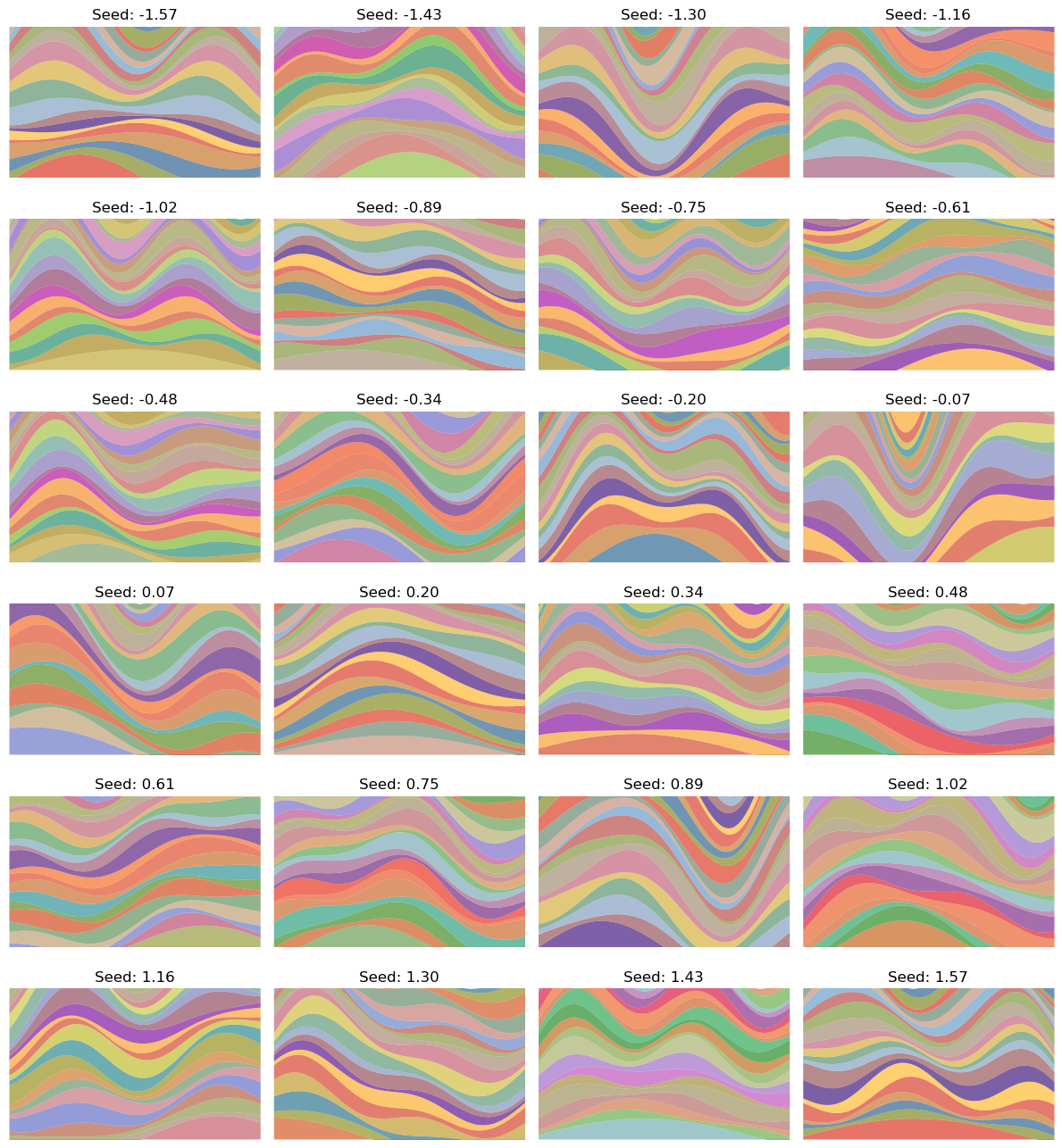
To be clear, there’s no randomness here, it’s just mapping $t \in \mathbb R$ to these different images, and if I rerun it with the same $t$ value, it’ll produce the same image again. And I’m pretty confident that A) it’ll never make the same image twice, and B) the “invalid” image I made above won’t ever get produced.
Skipping over a few details, here’s what I did:
- the $i$th band is specified with three parameters:
- $t_i$, the thickness
- $f_i$, the frequency
- $\phi_i$, the phase
- each image is a stack of $N$ bands, so $3N$ parameters specifies one of these images
- and due to how the bands stack, two different sets of $3N$ parameters will lead to different images
- I map $t \in \mathbb R$ to the range $x \in [-\pi/2, \pi/2]$ with $x = \frac{\pi}{2} \tanh t$
- I map $x$ to the unique vector $v = [\sin x, \sin p_1 x, \sin p_2 x, \dots, \sin p_{3N - 1} x]$ of length $3N$, where the $p_i$ are the primes ordered
- I also make $x$ smoothly interpolate between a cycle of colors
Note that although some subsets of the components of $v$ will repeat for different $x$ (and therefore $t$), $x \in [-\pi/2, \pi/2]$, and the first element is always increasing with $x$ so the vector as a whole will never repeat.
Since I framed it in terms of being a 1D Gaussian distribution, you can basically just view $t$ as the support of it, and do this process for any samples.
Finally, note just how much diversity in the images got packed into the single dimension of $t$. In fact, when I went to make the gif below to visualize “scanning” across the $x$ values as in the grid above, I first made it vary $x \in [-\pi/2, \pi/2]$, but found that the image parameters change so quickly over the whole range that it was basically a chaotic mess of unrelated looking images! I changed it to $x \in [-0.1, 0.1]$ which was still too wide, so went with $x \in [-0.01, 0.01]$, which produces:
Still changing a ton in that tiny region.
But… the game?
This was obviously a silly example of what I wanted to illustrate (and an excuse to do it with pretty pictures), but could the approach I described above practically solve this? I.e., could we train a VAE/etc to take these $\approx 5 \times 10^5$ dimensional images and embed them into a 1-dimensional space? Even if we were given a massive dataset of them?
It’s an interesting question and I’m not quite sure how to think about it. My guess is “no” in a practical sense, even if it theoretically should be possible with enough model capacity and training data.
A couple thoughts off the top of my head:
Even when a manifold is 1D in some higher dimensional space, there’s still definitely a range of complexity the manifold can have in that space. For example, the 3D helix-like one I made above is definitely more complex than a simple 1D line embedded in 3D space, even if they’re both 1D manifolds. And, I’m guessing the line is a lot easier to transform back to 1D than the helix is. I’m not sure what property would distinguish these, maybe mean curvature?
In a similar vein, the other thing I was thinking was that in what I’ve said above, I’ve been assuming that the raw data being in a higher dimensional space makes the job of transforming back to the lower dimensional space harder on average; that just seemed intuitive. But now I’m thinking: maybe that’s not true?
Here’s some iteration of a Hilbert curve:
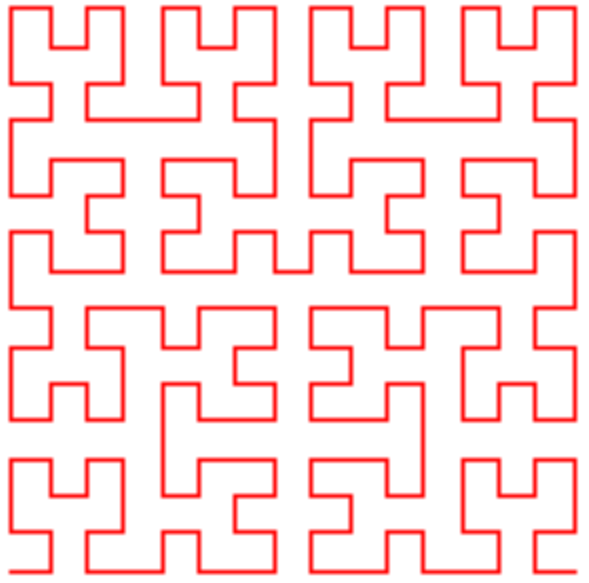
which we could view as a 1D manifold in 2D space, if it was smooth, etc. You can get a lot of mileage out of the “deep learning as stretching and folding space” analogy. It seems like it’d be pretty brutal to have to unfold that mess and map in onto a line in 1D, and it certainly seems harder than many simpler 1D manifolds in 3D. But what I’m wondering here is, is it partially harder because it’s only in 2D space?
I.e., if we imagine the Hilbert curve above but stretched out into a third dimension (but to be clear not a 3D Hilbert curve, just the shape above but with some variation in the 3rd dimension), it seems plausible that it might actually be easier to do the necessary transformation. As an extreme example, imagine the curve has been stretched out in the 3rd dimension so that the beginning of it has a really negative $z$ value and the end of it has a really positive $z$ value – then the work is basically almost done.