GCRL - extras
Last time, I talked about some of the motivations for doing MTRL, and specifically GCRL. Today, I’ll go into a bit more depth about a few aspects and give some thoughts about different approaches.
Today the focus will be almost entirely on GCRL specifically, where the extra input is a goal in some form. For reasons you’ll see in a minute, I’m also going to use the symbol $g$ for the goal conditioning variable rather than the $z$ we’ve been using so far.
It’s all about the embeddings, baby
I have to come clean with you: I’ve been hiding a big aspect of many GCRL algorithms. Notably, embeddings.
You can do GCRL as I’ve described it up to this point without dealing with embeddings just fine. If we drew block diagrams for the stuff I’ve described so far, they might look like this:
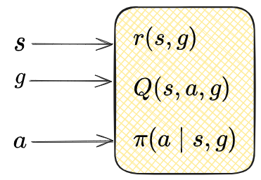
I.e., we basically do the normal stuff, but just have an extra $g$ input that determines the goal.
However, for “real” problems and fancier research topics, people often need to use or manipulate the state in some way, and it can be really tricky for various reasons to do this with the raw observations. Therefore, it’s very common in GCRL to “embed” (or “encode”, you’ll see either used interchangeably) the raw observation into an intermediate form that alleviates these problems.
If the raw observation is $s$, and the embedding function is $\phi$, then it’s very common to write the embedding of $s$ as $z = \phi(s)$. Yeah, it sucks that $z$ is used for this also here. Sorry.
Below I’ll go over two big reasons embeddings are used in GCRL, but it’s really the tip of the iceberg.
Rewards
Last time when I mentioned some of the problems GCRL has, I gave an example of the commonly used “dense” distance from the goal reward function, $r(s, g) = -\Vert s - g \Vert^2$. There, I pointed out that it doesn’t make a lot of sense if your state contains features with different units and types of measurements; some quantities just aren’t comparable.
The problem gets even worse though when you consider having raw images as inputs! With image inputs we don’t even have features, so the issue about units or scales is irrelevant. The problem with image inputs is that the aspects that determine the difference between states are high level contents of the image, like “is the dog inside the doghouse or on top of the doghouse?”
I wrote about this here with some examples, where I allude to our current scenario at the end. Basically, you can handle images by training an embedding $\phi(s)$ that maps raw observations to a latent space, where your rewards and models operate from. So now the block diagram above might look like:
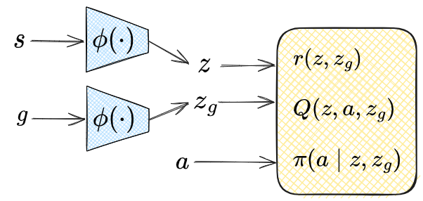
You may have noticed that I motivated this with discussion of the reward, but didn’t actually say what form the reward takes after embedding. That’s in the next big section below so read on!
Similar states
The other big reason to use embeddings stems from a similar cause as the rewards issue above, but with a different effect.
In many GCRL methods, we need the ability to produce possible goal states (without going into detail, they’re often used for either speeding up the learning process, or used for forward planning). That is, we need to be able to sample states that are ones that the agent might actually see, and ideally, have the ability to produce ones that are similar or relevant to another state (such as the agent’s current state).
How might we do this? Naively, if our state were an $N$-dimensional vector, you could try just changing the value of one of the dimensions, or adding some Gaussian noise to all dimensions, etc.
However, a similar issue to the rewards one above arises: the states are very high dimensional, but the valid states are fundamentally of a lower dimension. This makes naively changing the values of valid states produce states that are probably invalid, and makes modeling their distribution in the original high dimensional space really hard. I wrote about it here, with some nifty figures to illustrate it.
And like I mention at the end of that post, the common approach is to learn a transformation between the original high dimensional space and a lower dimensional space that the valid states fill. Or, you might call it… an embedding.
GCRLilocks and the three reward functions
As mentioned above, part of the motivation for using embeddings is to be able to make sensible GCRL reward functions. But what should they actually be?
There are a few commonly used ones in GCRL. In what I say below, even if we’re using an embedding $\phi$, I’m still just writing $s$ and $g$, but they’d really instead be $\phi(s)$ and $\phi(z)$. I’m also glossing over some “off by one” issues here about which state you receive the reward for, etc.
As an illustrating example, let’s look at a simple 1D chain Markov reward process:
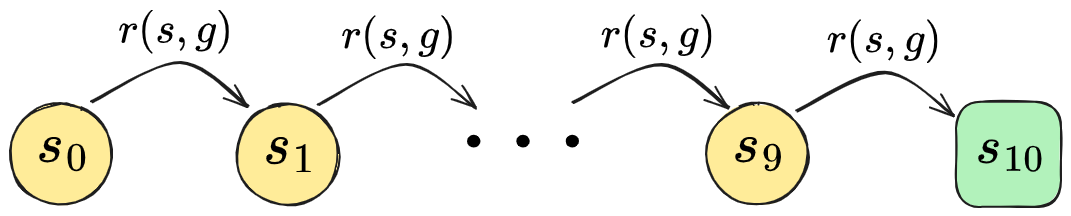
I.e., there are no actions, it just deterministically starts off in state $s_0$ and each step goes to the next state until it reaches $s_{10}$ and the episode ends. And, we’ll just consider the case where the goal is $g = s_{10}$.
I’ve plotted a few commonly used GCRL reward functions and their resulting VFs as a function of the state index, below, which I’ll refer to. This is obviously different than real GCRL problems for a million reasons, but it’s simple enough that it’ll let us see the “shape” of them.
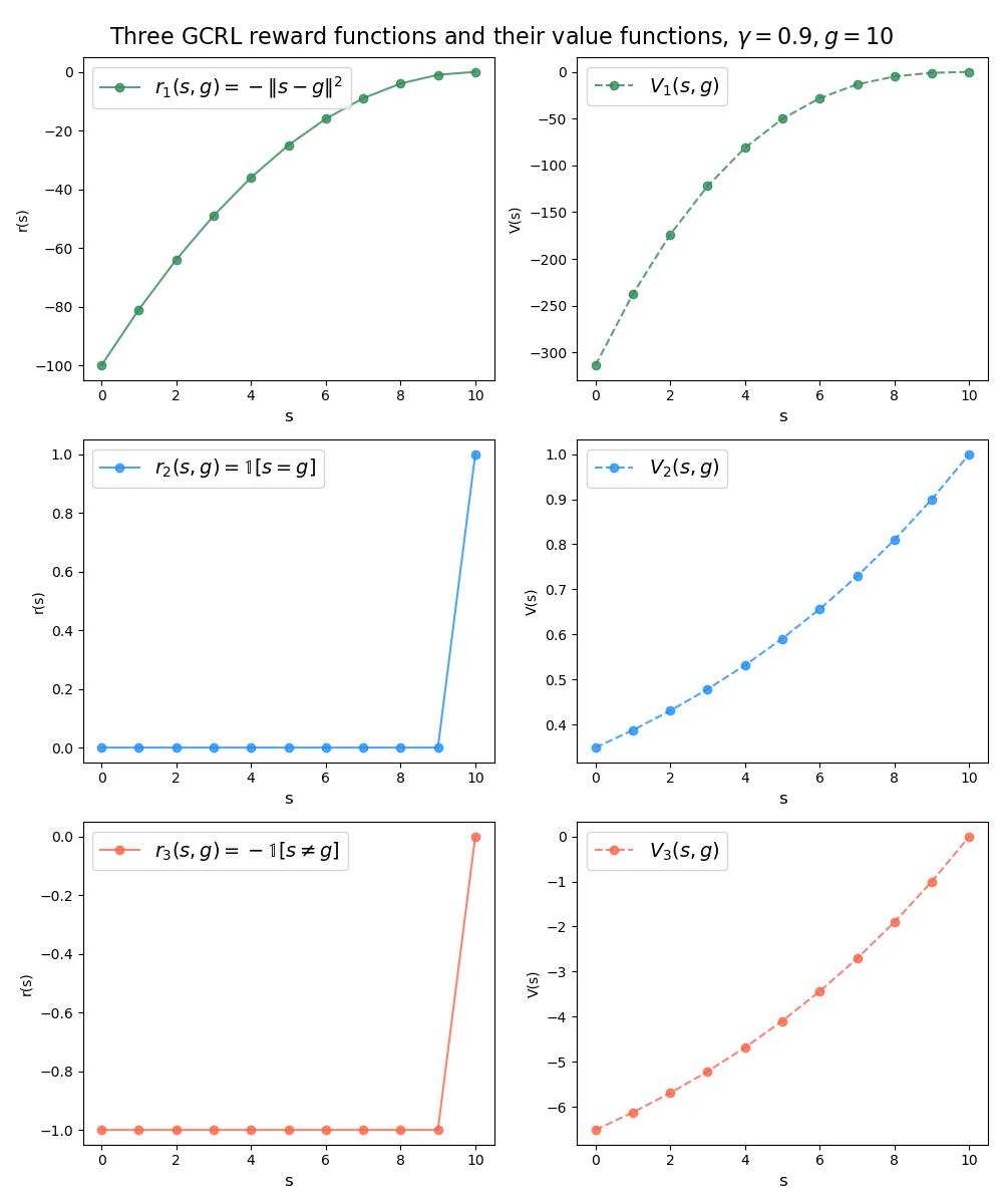
The first reward function is the “dense” one, $r(s, g) = -\Vert s - g \Vert^2$ (first row). This has the advantage that it’s, well, dense, so you’re always getting a reward signal. However, it probably won’t work well unless either the state space is simple enough that the $s-g$ delta is meaningful, or we define an embedding (and therefore make $\phi(s) - \phi(g)$ meaningful). It could also be an issue that $r$ grows (negatively) without bound as $s$ gets really far from $g$; the GCVF is going to have to model these values, and it can cause trouble when it’s forced to cover a wide range of values during all of training (you can see in the right column plot how quickly it’s growing). A related downside might be the same issue that naive gradient descent faces: as you get closer and closer to the goal, the gradient of the reward function gets smaller and smaller, meaning that the attractive force to get even closer to the goal diminishes.
The second reward function (second row) is maybe the most straightforward, the sparse “are you at the goal” indicator function $r(s, g) = \mathbb 1 [s = g]$. This basically has the reverse of the issues above: it’s sparse rather than dense, which can hurt, but its VF is bounded (you can see that the VF basically has the form $\gamma^n$, when it’s $n$ steps away from the goal). It also doesn’t have the problem of a slowing gradient near the goal: it really wants to get to the goal, since that’s the one place it’ll receive reward.
However, there’s something else worth mentioning. If you were to collect experience with the typical “sample a goal, condition the policy on it, and update the models conditioned on that goal with that experience” procedure, you might notice that unless the state space is both discrete and pretty small, it’s pretty much impossible that the agent will ever actually achieve $s = g$ exactly! For example, a robot arm whose goal it is to get to the configuration $g = (3.82, -1.50001, 5.1)$ probably won’t ever get those exact coordinates.
As you might guess, for both the dense reward function and this one, in practice it’s common to use an “epsilon-ball” done function, where the episode ends and it gets the reward when we say it’s close enough, i.e., $\Vert s - g \Vert \leq \epsilon$. However… you might also notice that this is going to run into the same issue as the first one! I.e., you need an embedding to meaningfully compare $s$ and $g$ for this. There’s one interesting wrinkle to this: if you do relabeling, you wouldn’t need an embedding to do this – any trajectory you relabel will necessarily be relabeled to have $s = g$ exactly, and you can do backups from that.

The last reward function (third row) is almost the same as the second one, but it seems to be more common and has a slightly different interpretation. It’s basically the second one, but minus one; explicitly, $r(s, g) = -\mathbb 1 [s \neq g]$, or, “negative one reward every step until you get to the goal”. And as you can see in the plots, if you squint until the axes labels are blurry, both its reward function and VF have the same shape as the second one.
Why distinguish them then? Well, partly because I’m just reporting the facts on what people use :P but there might be good reasons. One difference is that for the 3rd reward function, $V(s, g)$ will represent the (negative) “temporal metric” between states, $d(s, g)$; i.e., the (discounted) number of timesteps to go from $s$ to $g$. There’s a history of metric modeling methods outside of RL, and there are some active and pretty interesting research threads that are using these methods to learn a VF with these properties. In contrast, the VF for the 2nd reward function will also be kind of metric-based, but will instead be $V(s, g) = \gamma^{d(s, g)}$.
Another obvious difference is that the VF for the 2nd will be bounded to $[0, 1]$, while the 3rd can be (practically) unbounded in the negative direction. Usually I’d say being potentially unbounded is worse, but they’re very differently shaped function and it’s possible one is better than the other because of that.
Which brings me to my last point. Without going into the whole ball of worms that is discounted vs undiscounted RL, if we take the limit as $\gamma \rightarrow 1$, the VF for the 3rd RF will approach the actual, undiscounted (negative) metric, i.e., $V(s, g) \rightarrow -d(s, g)$. This will still clearly be useful for learning. But in the same limit, the VF for the 2nd RF will approach…. $1$, at all states that are capable of reaching the goal. And that won’t be super useful for learning a policy. I dunno, I need to think about this more, maybe I’m missing something.
The different ways $z$ gets used
Like I mentioned in the first post in this series, these methods are all birds of a feather and kind of the same if you’re willing to be reductive enough. I.e., at the end of the day we input some extra variable to our policy and it should act differently. But of course, people are doing slightly different things with them and give them different names based on that.
The main aspects that distinguish them are what rewards get used, and as an extension, the “meaning” behind the conditioning variable (I’ll just stick with $z$ here). I’ll briefly go over these.
MTRL
This is the most general and in some sense encompasses the others, but I’ll talk about it here to mean the case where we’ve designed some reward function $r(s, a, z)$. $z$ could be a single scalar or an $N$-dimensional real vector with a reward that changes continuously with $z$, or a one-hot or multi-hot vector with totally separate reward function terms that are “activated” by $z$ being “on” on “off”. I mean, this is so general that the world’s your GCRL oyster.
A good example would be the work in the Meta-world paper, where they are training a bunch of (simulated) robots, and if you look at the appendix (see pics in last GCRL post), they have a big ol’ list of nasty, hand defined reward functions. They activate them with the different values of $z$.
The main point here is that what $z$ “represents” is just kind of a general control knob, and there’s no inherent meaning besides what you’ve designed in.
GCRL
This is the more specific case I’ve mostly been talking about, where $z$ corresponds to a goal state, whether it’s a literal state or a latent state (I’m distinguishing between those here, because a latent state almost certainly corresponds to more than one literal state in most practical cases). So although we have choice in how we want to represent the state for the models, GCRL is somewhat constrained in what the conditioning variable means.
Similarly, although you of course can do whatever the hell you want, in GCRL the reward functions almost always reflect some interpretation of a distance. A classic paper that is almost synonymous with GCRL for many is the UVFA paper from 2015.
USD
Unsupervised Skill Discovery (USD) is super cool, and fits into this paradigm but in a slightly different way. Most USD methods also use a conditioning variable $z$, but in contrast to the niches above, in most USD methods $z$ isn’t something you get to define the meaning of (as in MTRL) or something that has an inherent meaning (as in GCRL, where it’s connected to the state). It’s more… discovered. Let me explain.
The main idea behind USD is that there are inherent behaviors (or “skills”) in the environment that can be discovered, in an… you guessed it, unsupervised way. For example, forgetting about any concept of a reward function, there are distinctly different ways of acting in a given environment if you explored what you can do in it fully. For example, while there’s the typical way to ride a bicycle, people also develop all sorts of crazy skills with bikes, like doing a wheelie, halfpipe tricks, acrobatics, riding backwards, etc. Those skills kind of just inherently exist in the “riding a bike” env.
USD trains an agent to find those skills, without having to provide a reward signal for them specifically. In USD, $z$ defines a “skill space”, and there’s usually a $z$-dependent “pseudo-reward” that’s maximized by the agent acting in ways that make it easiest to distinguish which $z$ is currently being used. In the simplest example, the pseudo-reward can be based on a discriminator model $q(z \mid s)$. This encourages the policy to “partition” the state space such that for one $z$ value, it only visits some states, and for another $z$ value, it visits a different set of states, etc. This is exactly what they do in “Diversity Is All You Need” (this was in 2018 when “X is all you need” hadn’t completely jumped the shark yet), a canonical USD paper that really kicked off the recent trend of them.
Getting back to the reason I brought this up, this causes $z$ to be a bit different than the other niches. If the USD algo is successful, conditioning the policy on different $z$ values will give different behaviors, but you don’t get to choose A) what behaviors they are, or B) which $z$ value will correspond to a given behavior. It’ll just be this “soup” of behaviors corresponding to different $z$ values.
Why train one model instead of several?
I think it’s always good to ask the “why don’t you just do X” question. Not to be anti-progress or anti-trying-things, but to see what really makes some technique work well. So in this case, it’s worth asking: why are we doing this all with one model? That is, why not use different NN models for different tasks (in MTRL) or skills (in USD), or maybe even goals? Let’s focus on simple MTRL for now.
The common MTRL case where $z$ is one-hot and corresponds to fairly different reward components seems like a scenario where this question could especially apply; if the tasks are that different, why are we trying to cram them together into one model? Why not just have $N$ models for $N$ tasks?
Straightforward reason: fewer models
The most straightforward reason is just that if we can avoid it, we’d rather just have one model than $N$ of the same size, for any number of reasons (memory, for example). And, if $N$ is large, it’ll actually be infeasible to have $N$ models.
But this only partially answers it: first, in some cases, people aren’t actually doing such a large number of tasks that it’d be infeasible to have a model for each. In that case, it might be simpler overall to just have $N$ models and a single-task setup. Second, it’s unlikely that the multi-task models will actually be the same size as a single task one; NN capacity isn’t free, and the more different the tasks are, the bigger the multi-task NN might have to be.
Generalization magick
An answer you’ll usually see in papers is GENERALIZATION. I.e., if we learned the tasks separately in different models, each model would only be trained by the experience for its corresponding task, whereas with MTRL in a single model, you’ll get a magic GENERALIZATION multiplier where optimizing the model for one task will learn representations that are still useful for the other task.
And this makes some sense intuitively, right? Lots of skills in real life have transferability between them. But in RL practice… I dunno. One immediate red flag is that there’s a whole sub-niche of MTRL papers about combating what’s called “task interference”, which is exactly what it sounds like, where it’s harder to learn multiple tasks simultaneously. I’m not saying multi-task generalization can’t speed up learning, I’m just saying that it seems like the opposite is empirically happening at least sometimes.
To quote the Meta-world paper:
While having a tremendous impact on the multi-task reinforcement learning research community, the Atari games included in the benchmark have significant differences in visual appearance, controls, and objectives, making it challenging to acquire any efficiency gains through shared learning. In fact, many prior multi-task learning methods have observed substantial negative transfer between the Atari games. In contrast, we would like to study a case where positive transfer between the different tasks should be possible. We therefore propose a set of related yet diverse tasks that share the same robot, action space, and workspace.
So basically, if the tasks are too different, it’s known that it starts to hurt, but they aimed to use ones that would hopefully help.
Curse of dimensionality (also generalization)
Another reason also kind of relies on generalization as an argument, but in a different way. Let’s assume that our MTRL $z$ variable is now composed of two concat’d one-hot vectors, $z_1$ and $z_2$, each of length $N$. For example, $z_1$ controls what room your cleaning robot will clean, and $z_2$ controls what cleaning tool it will use. So now there’d be $N^2$ unique combinations of the $(z_1, z_2)$ values.
Since this will scale exponentially with the number $T$ of different types of settings you want to have, we’re clearly not going to have $N^T$ models, and then the straightforward first reason above would apply.
However, you might notice a wrinkle here. We’re using a single model that learns to do all the $N^T$ combinations of tasks because it’d be infeasible to have that many models, but we still have to actually get experience from doing these different tasks to train this mega-model. If $N^T$ is that massive, there’s no way we’ll be able to collect enough data for each task (sure, relabeling will help some if you can do it, but… $N^T$).

The real answer is that this is also gonna rely on some form of generalization happening. The only way this is really going to work is if the different one-hot vectors for a given $z_i$ only change the reward in a relatively “separable” way. As a simple example, if it has never seen data for the specific example: \(\displaylines{ z_1 = [0, 1, 0, 0, 0, 0], \\ z_2 = [0, 0, 0, 0, 1, 0] \\ }\) but it has seen data for $z_1 = [0, 1, 0, 0, 0, 0]$ and other values of $z_2$, and has seen data for $z_2 = [0, 0, 0, 0, 1, 0]$ and other values of $z_1$, and in this environment that knowledge actually does help determine the rewards for the specific yet-unseen $(z_1, z_2)$ values above, then the model should be able to learn to “generalize” and handle all the different cases, even ones it has never trained on.
This seems like it could plausibly happen in some practical problems (e.g., if the cleaning robot knows how to get to and move around the kitchen, and it has learned to sweep in the bathroom, it seems reasonable that it could generalize to sweeping in the kitchen even if it never trained specifically on that). But, note that there’s nothing that says this has to be the case. The reward function could totally change in a nonlinear, non-smooth way such that changing the value of $z_1$ from $[1, 0, 0, 0, 0, 0]$ to $[0, 1, 0, 0, 0, 0]$ has a completely different effect when $z_2 = [0, 0, 0, 0, 1, 0]$ compared to when $z_2 = [0, 0, 0, 0, 0, 1]$.
What are you supposed to do in that case?
¯\_(ツ)_/¯
I mean, at that point we’re kind of just asking it to learn $N^T$ very different problems, so I don’t think we can expect much a standard model free, MTRL algo to somehow learn all of them.
That said, there are still some approaches that could help a bit. Even if these different reward functions are incentivizing very different behaviors, they still exist in the same environment with the same dynamics. So that could still be leveraged, either through MBRL or GCRL. However, as I mentioned last time, you’d still need to either solve for the optimal policy (for MBRL), or figure out which states to traverse to for different rewards (for GCRL). So it’s not like they solve it either.
Alright, that’s all for the main GCRL posts! Soon, I’ll follow up with some posts on more specific papers and techniques, and then some experiments of my own, and refer back to this and the previous posts rather than explain there.