Meet the RIGs! An overview of the RIG family of GCRL algorithms

In a few recent posts, I discussed the background, motivations, and some details about Goal Conditioned Reinforcement Learning (GCRL). Today, I’m looking at a specific family of GCRL algorithms that I think are pretty cool. There are a bunch of them, and I would’ve found it useful if I could’ve read an overview like this when I was digging into them, so hopefully it can help someone else.

The RIG picture

The reason I call these the “RIG family” is that the first paper’s acronym is “RIG”, and the following papers all basically do variations and improvements on the same core idea, namely, to embed high dimensional (usually image-space) observations into a lower dimensional latent space, and then generate goal states in that latent space. In my opinion, there are two main motivations for this: to help with either/both 1) learning a GC policy (GCP) and 2) planning.

Learning motivation

The learning motivation can be further broken down into two main parts, below.

Generating “practice” goals

Since these are all GCRL methods, a big part of that is training the models to, you know, achieve goals, and part of that is having goals to attempt. However, in real environments it’s not trivial to produce meaningful goals. Goal relabeling is helpful, but ultimately it’d be better if we could produce entirely new goals for the agent to try and achieve. These methods operate in the latent space, where that task is easier.

Making a good GCRL reward

As I discussed previously, it’s very common in GCRL to use rewards that correspond to a (negative) distance (literal or abstract) from the current state to the goal state. However, doing this naively also won’t work in real environments; briefly, distances in the raw observation space often have no relation to their actual distance from the goal (e.g., if a robot’s observations are images, and its goal is an image of its viewpoint while being in the living room, dimming the lights will change the image massively despite it being at the goal).

Planning motivation

Planning is (generally) a separate axis from RL, although it can be used to assist the RL training, and can certainly leverage the RL models. For the papers in this post, it’ll usually mean the scenario in which the desired goal is distant enough from the agent’s current state that we can’t simply plug the goal $g$ into our GCP (e.g., $\pi(s, a, g)$) and expect it to get there. To handle this, it’s common to optimize a sequence of subgoals between the current state and goal state that should be easier to go between. Like generating the practice goals above, this is much easier if the subgoals are in a compact, structured latent space.

Themes and differences

These papers all work off the same core ideas, but they are different enough to put in separate papers. Distilling their thematic differences down to a short bullet list, they’d be something like:

• Goal sampling: unconditional vs conditional sampling.
  • When sampling a goal, you can either sample any state from your data distribution (unconditional), or you can sample states conditioned on something (usually your current state).
• Goal generation: single goals vs subgoal sequences.
  • A few of the papers are concerned with just generating one goal to achieve, while others are concerned with generating a sequence of (sub)goals.
• Subgoal feasibility: simple latent distance cost vs using the value function.
  • To choose between different sequences of subgoals from an initial to a final state, we need to determine the difficulty of getting from each subgoal to the next one. A simple way is to use the distance in the latent space, but a better way could be to use the VF.
• Method of traversing between subgoals: learned policy vs MPC.
  • Once a subgoal sequence has been chosen, you need to actually go from one to the other. Most of these methods use the GCP they’re training, but you can also use an MPC (which will require a model).

Comments up front

The publish dates for the papers aren’t exact. I think I just took the ones from the arxiv pages. But they’re roughly in chronological order, since they do build upon each other.

The authors are a bit of a rotating cast. Professor Sergey Levine is the common thread to all of them, but there are a few other repeat characters: Chelsea Finn, Ashvin Nair, Vitchyr Pong, Steven Lin, Patrick Yin, and probably a bunch of others I’m missing.

I’m gonna try and keep this short. To do that, I’ll discuss the initial RIG paper at some length, but for the others I’ll just highlight the similarities and differences of them with respect to the ones that came before.

Let’s meet them!

RIG (2018)

RIG stands for “RL with imagined goals” and comes from “Visual Reinforcement Learning with Imagined Goals”.

RIG is the simplest of these methods and is only concerned with the two parts of the “learning aspect” I mentioned in “the RIG picture” above. It’s probably best to just jump in. Here’s the high level overview of what RIG does:

• Start with a bunch of raw data, or use an exploration policy to collect some
• Train a VAE to learn an embedding of this data into a latent space $z$
• Online RL training:
  • Have a policy $\pi(z, z_g)$ and Q function $Q(z, a, z_g)$ that operate on the latent space
  • At the beginning of episodes, sample a goal from the VAE prior $p(z) \sim \mathcal N(0, 1)$, and plug this into the policy so it’ll try and achieve that goal
  • Use the VAE encoder to convert raw observations $s_i$ into their latent values: $z_i = e(s_i)$
  • Each step, calculate a reward based on the distance in the latent space between the current (latent) state $z$ and the latent goal state $z_g$: $r(z, z_g) = -|z - z_g|$
  • Some fraction of the time, do HER-style relabeling of the achieved goal
  • Train the RL models based on this reward

Why do they use the VAE, exactly?

We learn a visual representation with three distinct purposes: sampling goals for self-supervised practice, providing a structured transformation of raw sensory inputs, and computing a reward signal for goal reaching.

The 1st and 3rd ones are the important parts:

• If the VAE is learned perfectly, then it has captured the true data distribution well and transformed it into the prior distribution in the latent space. So, sampling from its prior should give latent states that correspond to only real, plausible looking states, ones that we’d like the policy to try learning to get to.
• The form of the reward is intuitive enough: it’s the negative distance from the current state to the goal state, so to maximize the reward you’d want to get that distance close to zero, i.e., get as close to the goal as possible. However, as I’ve talked about in other posts, if you naively took the distance in image space, it wouldn’t reflect a distance at all. However, calculating the same distance in the latent space should act a lot more like a distance.

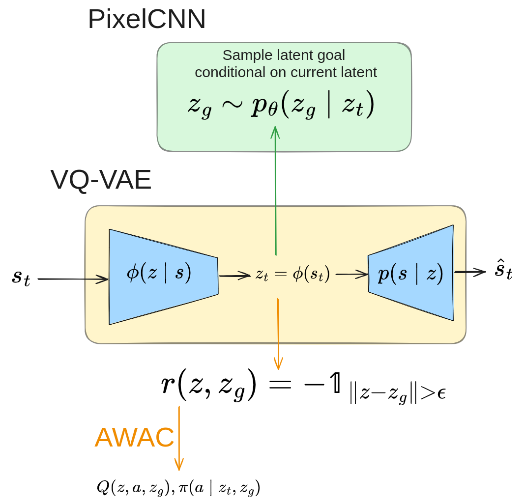
Here’s my diagram that puts it all together for me:

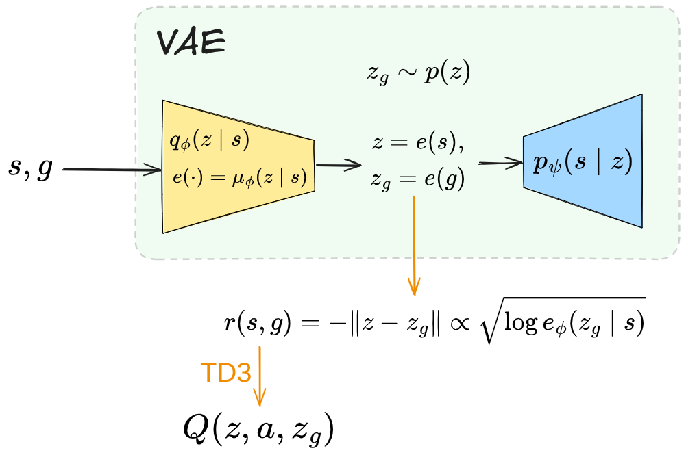
They use TD3 to learn the RL part. This choice isn’t super important, which is a theme with a lot of these GCRL papers: it’s more about some other scaffolding around the RL. There are some more details and thoughts, but you can read about those in the “extras” section at the bottom.

CC-RIG (2019)

CC-RIG stands for “Context-conditioned RIG” and comes from “Contextual Imagined Goals for Self-Supervised Robotic Learning”.

CC-RIG is nearly the same as RIG, but introduces conditional goal sampling, a big improvement that most of the following papers also do.

Similarities to previous

• Uses a (type of) VAE like RIG

Everything else is pretty similar to RIG: The CC-VAE is trained before any RL part. The reward is the same latent distance one as RIG, and they use TD3 again.

Differences from previous

• The VAE is a (type of) CVAE instead, so does conditional goal sampling

The main motivation of CC-RIG is about a shortcoming of RIG: in RIG, since the VAE (hopefully) models the distribution of all states in the dataset, sampling a goal state might give you any state – but not necessarily one that’s reachable from the current/initial state.

For example, if the episode starts with a robot arm and a green block on the table (and assuming the robot can’t add or remove blocks), it’d be an impossible task if the sampled goal had a red block in some orientation.

CC-RIG aims to overcome this by using a type of conditional VAE (CVAE) they call a CC-VAE, instead of a plain VAE. With the CC-VAE, the encoder and decoder are both conditioned on the “context”, which is basically the initial state of the episode. Therefore, the CC-VAE is now trained on pairs $(s_0, s_t)$ of observations from a trajectory, where $s_0$ is an earlier state and $s_t$ is a later state. $s_0$ is the context, the conditioning variable, so as in a typical CVAE, it’s trained to reconstruct $s_t$ and keep the latent $z_t$ close to the (Gaussian) prior.

The key point here is: because it’s conditioning on $s_0$, this conditional distribution will only produce states that can follow, and therefore be a valid goal for, $s_0$. Therefore, if we plug in the episode’s initial state as the context and sample from the prior, instead of getting any random state, we should only get states that could plausibly be achieved from $s_0$.

They have this helpful example figure:

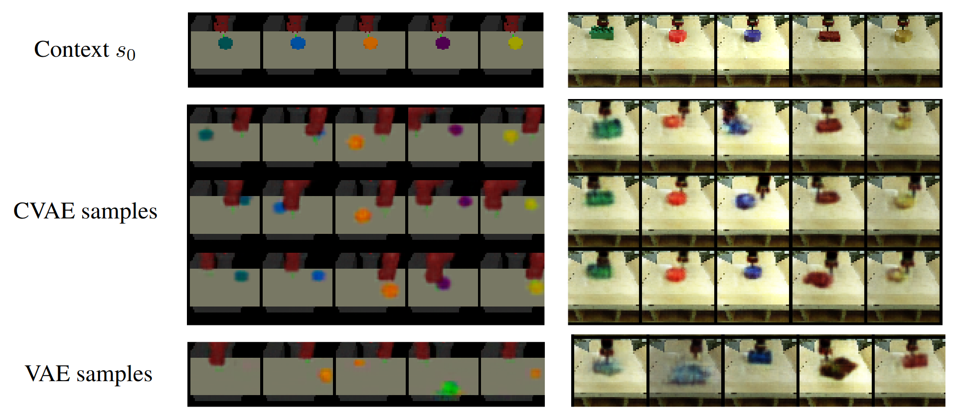
You can see that the VAE samples (bottom row) don’t seem achievable from the context in the top row (the block color changes), whereas the CVAE samples seem like plausible following states.

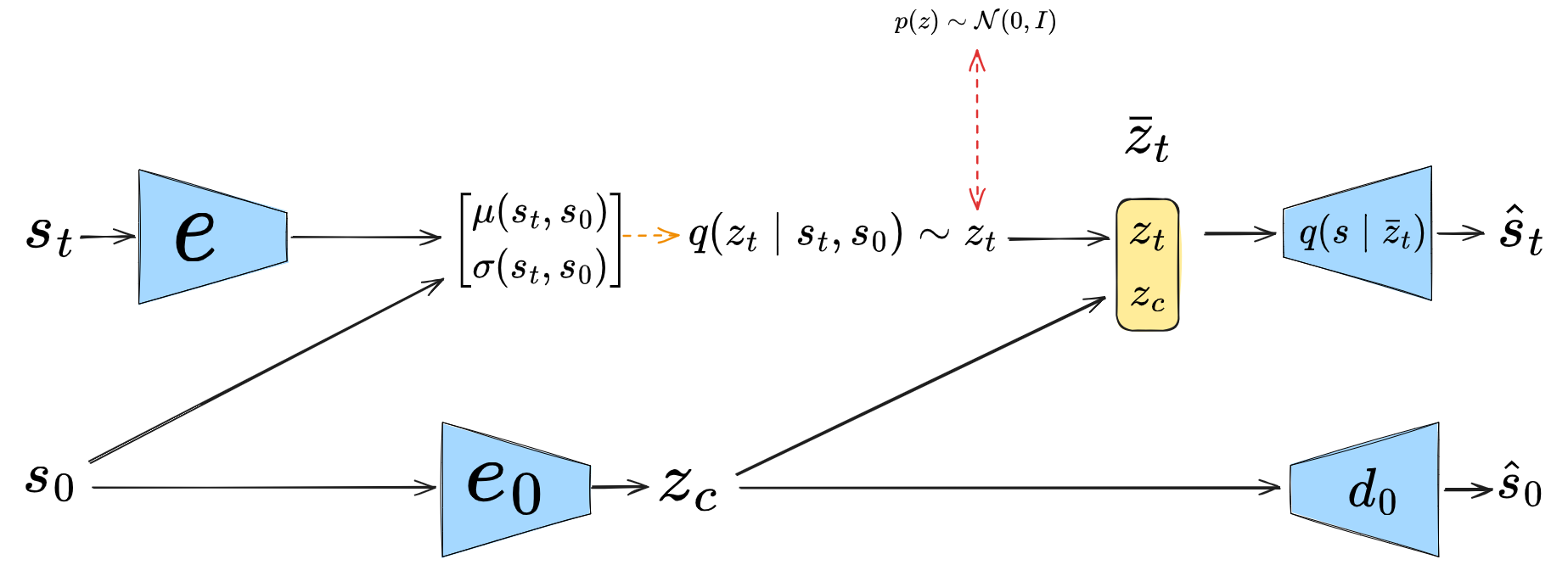
They have a diagram of the CC-VAE, but I actually found theirs a bit unclear, so I made this one:

LEAP (2019)

LEAP stands for “Latent Embeddings for Abstracted Planning” and comes from “Planning with Goal-Conditioned Policies”.

LEAP builds off of RIG, but explores a different axis than CC-RIG, notably planning.

Similarities to previous

Much is exactly the same as RIG:

• It trains the same simple (unconditional) VAE as RIG
• It uses the same dense “latent distance from goal” reward as RIG
• It trains a GCP and GCVF on this reward, like RIG

Differences from previous

• Generates subgoal sequences rather than just single goals

The problem it aims to solve is as follows: after the RIG-like training, in theory we should be able to plug any goal into our GCP and it should be able to go to it. Unfortunately, GCPs still don’t do great if the goal is really far away (in terms of number of steps) from the current state; they work best for short horizons.

So, a standard approach is to break down the task of navigating to a faraway goal into a sequence of several smaller “subgoals” in between the start and goal states. Since the subgoals are closer to each other, if the GCP can do those short segments well, it should be able to do the whole thing. This is a common theme in these papers.

That leaves one question: how to select the subgoals sequence? It has to be feasible to actually go from one to the other and eventually reach the goal. This is their clever contribution. Since it’s assumed that the RL training above produced a GCVF $V(s, g)$ and it’s relatively reliable for short horizons, if we’re in state $s$ and there’s a nearby state $s’$, plugging them in as $V(s, s’)$ gives us a measure of how easy it is to get from $s$ to $s’$.

Therefore, if we have a current state $s$, a faraway final goal $g$, and a sequence of subgoals $g_i$, $i \in 1, 2, \dots, K$, they define the “feasibility vector” as:

\[\vec{V}(s, g_{1:K}, g) = \begin{bmatrix} V(s, g_1) \\ V(g_1, g_2) \\ \dots \\ V(g_{K-1}, g_K) \\ V(g_K, g) \\ \end{bmatrix}\]

So, if we can find a subgoals sequence $g_{1:K}$ that minimizes (the norm of) this vector, each segment should be doable by the GCP, but only “aiming for” the current next subgoal. To optimize the feasibility vector, they just use CEM in the latent space.

HVF (2019)

HVF stands for “Hierarchical Visual Foresight” and comes from “Hierarchical Foresight: Self-Supervised Learning of Long-Horizon Tasks via Visual Subgoal Generation”.

This one is an odd bird compared to the others: it’s not even doing any RL! However, it’s using a bunch of the same elements, and it’s a good comparison point to see what the RL actually adds.

Similarities to previous

• Conditional goal sampling, very similar to CC-RIG
• It comes up with subgoal sequences, optimizing them with CEM, like LEAP

Differences from previous

• No RL, just online optimization!
• Trains a forward dynamics model

However, that’s where the similarities end. As I mentioned, it doesn’t do RL at all. It uses MPC to traverse between subgoals, and this of course requires a dynamics model, which they train. They also need a subgoal sequence score function for the CEM, but don’t have a VF to use the way LEAP did. So to score a proposed subgoal sequence, they apply the MPC to it, and use the MPC’s cost.

VAL (2021)

VAL stands for “visuomotor affordance learning” and comes from “What Can I Do Here? Learning New Skills by Imagining Visual Affordances”.

Similarities to previous

• Trains an unconditional VAE like RIG
• Trains a conditional goal sampler like CC-RIG

  Differences from previous

• They do some offline pretraining
• The VAE is a VQ-VAE
• Does the conditional goal sampling with another model, a pixelCNN

In VAL, they want to solve a similar problem as CC-RIG is, namely, generating meaningful goals from a given state. To do this, they… can you guess it? create a latent space embedding, using a VAE. At this point hopefully a pattern is starting to emerge.

However, VAL does it a bit differently: they train the (unconditional) VQ-VAE first, and then train an “affordance model” $p(z_g \mid z_0)$ to generate goals $z_g$, conditioned on the context embedded in the latent space, $z_0 = p(s_0)$.

Why might this be better? In CC-RIG, even though it’s good that goal sampling is conditioned on the (latent) context $z_0$, the goals for that context are still encouraged by the VAE objective to match a Gaussian prior, which can be pretty restrictive. Using a much more flexible generative model like a pixelCNN lets them generate goals for a context without having to satisfy that constraint. Here’s a helpful figure:

PTP (2022)

PTP stands for “Planning to Practice” and comes from “Planning to Practice: Efficient Online Fine-Tuning by Composing Goals in Latent Space”.

Similarities to previous

PTP and the following are where they really start doing a “kitchen sink” approach and combining a bunch of the elements from previous ones. It’s kind of a hybrid between LEAP and HVF.

• Conditional goal sampling, very similar to CC-RIG
• It optimizes subgoal sequences, like LEAP or HVF, but uses MPPI instead of CEM
• Uses the GCVF to score the feasibility of subgoal sequences, like LEAP
• Does offline pretraining, like VAL (though uses IQL rather than AWAC)

Differences from previous

• Recursive planning procedure

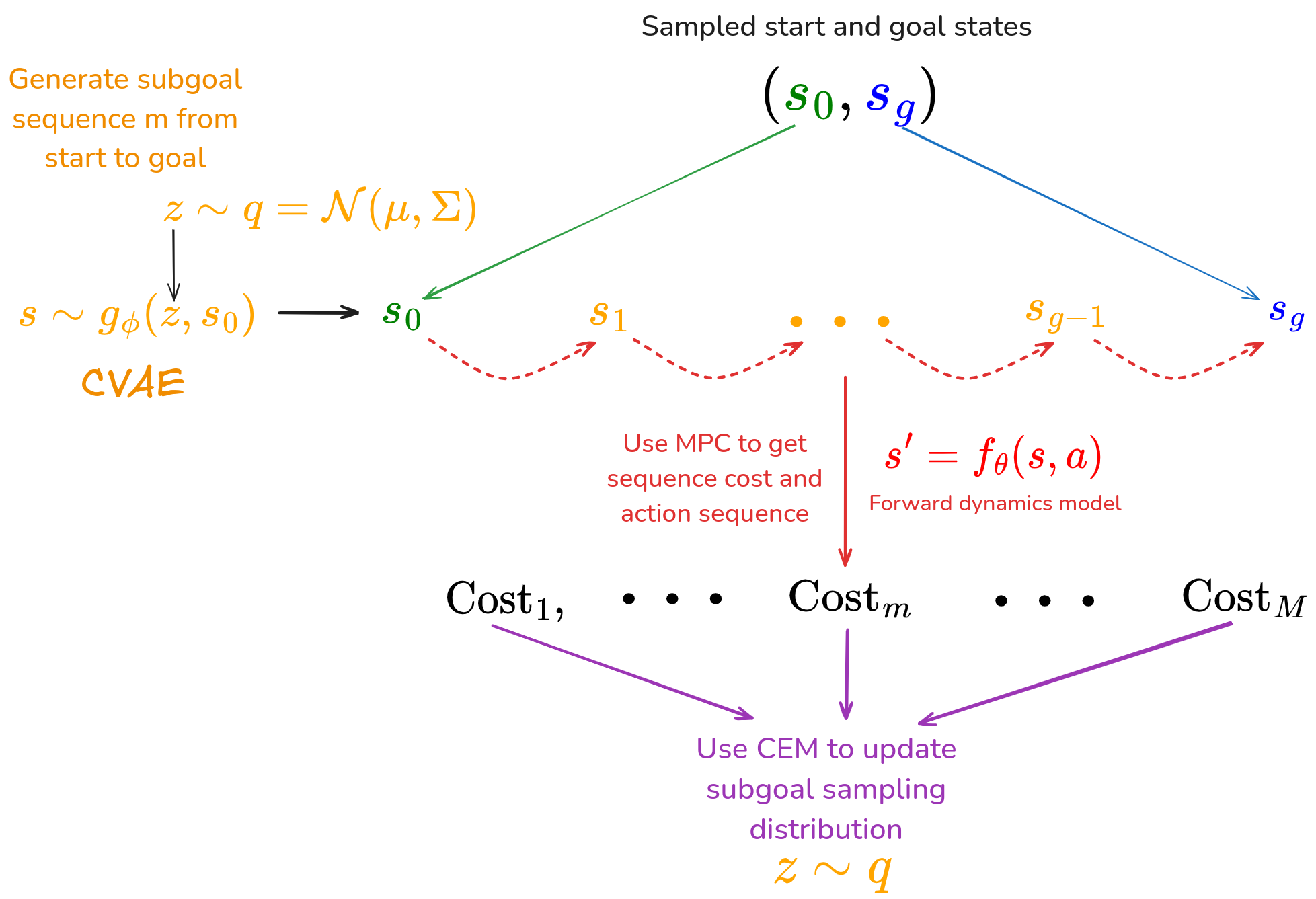
The main contribution of PTP is basically combining a bunch of threads from the previous papers, but also a recursive planning procedure. Without going too deep into the details here, here’s the main idea: in the previous works that optimize a subgoal sequence $s_{1:K}$ to a final goal, they typically just have a fixed number of subgoals $K$ between the current state $s_0$ and final goal $g$. That means that if $g$ is far enough away, even chopping it up into subgoals will still have the adjacent subgoal pairs $(s_i, s_{i+1})$ be pretty far apart, which it won’t do well with.

In the recursive planning idea, they call the planning subprocess $\text{Plan}(s_0, s_g, K)$ that produces a sequence of $K$ subgoals between $s_0$ and $s_g$. Then, in the initial call to $\text{Plan}(s_0, s_g, K)$ where it proposes $K$ subgoals $s_{1:K}$, they call $\text{Plan}(s_i, s_{i+1}, K)$ on each pair of subgoals, so it’ll produce $K$ subgoals between them, and so on. This ends at some depth level where the “finest” goals are a reasonably small distance apart that the GCP can handle them.

FLAP (2022)

FLAP stands for “Fine-Tuning with Lossy Affordance Planner” and comes from “Generalization with Lossy Affordances: Leveraging Broad Offline Data for Learning Visuomotor Tasks”.

Similarities to previous

FLAP follows up on PTP’s “kitchen sink” approach, even more so.

• Uses an “affordance model” conditioned on the current state to sample goals, like VAL (but, see below)
• Samples subgoal sequences recursively, like PTP
• Uses the GCVF to score subgoal sequences (optimizing with MPPI), like LEAP, PTP (but, see below)

Differences from previous

• The latent embedding simply comes from the offline RL training
• The affordance model is set up like a CVAE, rather than like the pixelCNN that VAL did
• In addition to using the GCVF to determine feasibility of the subgoal sequences, it also uses the probability of the $u$ that was sampled to generate the goal in the affordance model

One difference from previous papers is that here, the latent representation isn’t trained by a VAE/etc, but by using a common transformation $\phi$ for all their offline GCRL models (basically, like a shared NN layer). Here’s the figure from their paper:

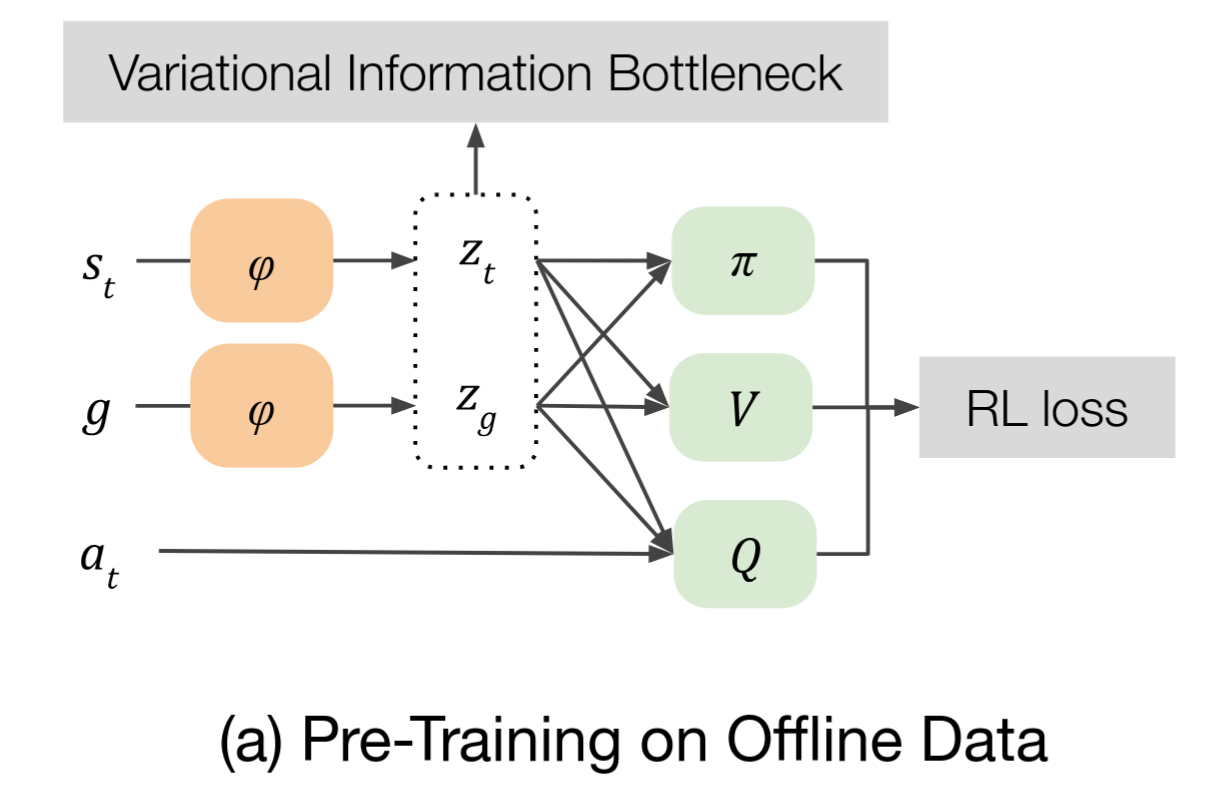
The transformation $z = \phi(s)$ produces the latent space, and it’s shared by all the models and updated in parallel as they’re learned. However, note the VIB part there – there’s a more in depth justification, but when the math cashes out this is basically a penalty on the typical RL loss, that incentivizes the latent representations $z$ to stay close to a Gaussian prior.

This might strike you as pretty similar to a VAE, which is no coincidence, because it’s done for a similar reason: so that we can sample the latent prior and hopefully be more likely to get latent values that actually correspond to real states.

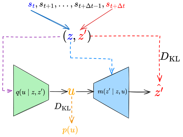
The other part that’s kind of new is their “affordance model” (AM). If you recall above, VAL (2021) also used an AM, where it used a pixelCNN to produce goal states from the latent value of the current state. In FLAP, the latent representation has already been produced by $\phi$ with the offline RL training, but they still want a way to do goal generation conditioned on the current state. To do this, they use a CVAE, like this figure I made:

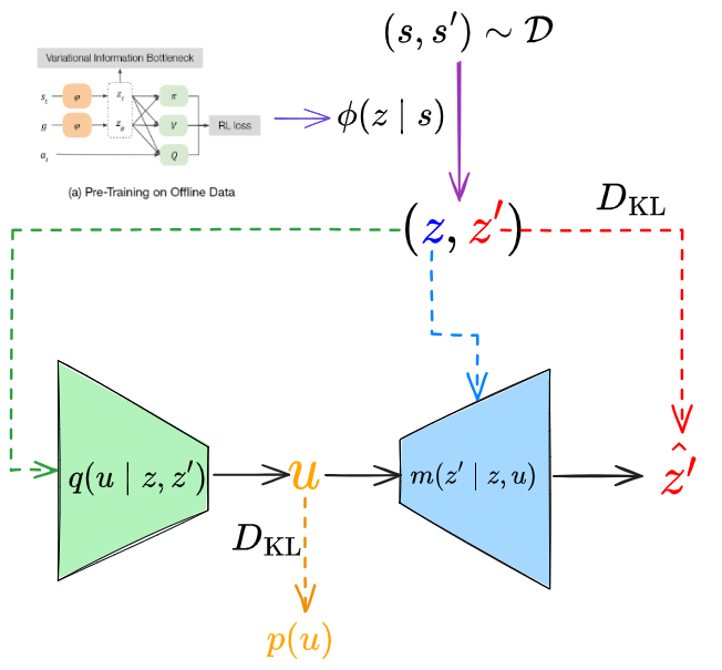
At first glance, this sure looks a lot like CC-RIG (2019). However, it’s actually different. In CC-RIG, the CVAE encoder is (effectively) $q(z_t \mid s_0, s_t)$ and the decoder is (effectively) $q(s_t \mid z_0, z_t)$. I.e., it’s used to produce the latent representation, and in a form that can produce plausible goal states for the context. The key point is that it’s basically going $(s_0, s_t) \rightarrow (z_0, z_t) \rightarrow (s_0, s_t)$ in a way that later allows you to sample from $p(z_t \mid z_0)$.

In FLAP, the AM CVAE doesn’t create the latent space of the states at all, since that’s already been created by $\phi$. Instead, the CVAE’s latent space is the variable $u$, which corresponds to a transition from $z$ to $z’$. So it’s basically doing $(z, z’) \rightarrow (z, u) \rightarrow z’$ in a way that later lets us sample from $p(z’ \mid z)$.

Wrapping it up

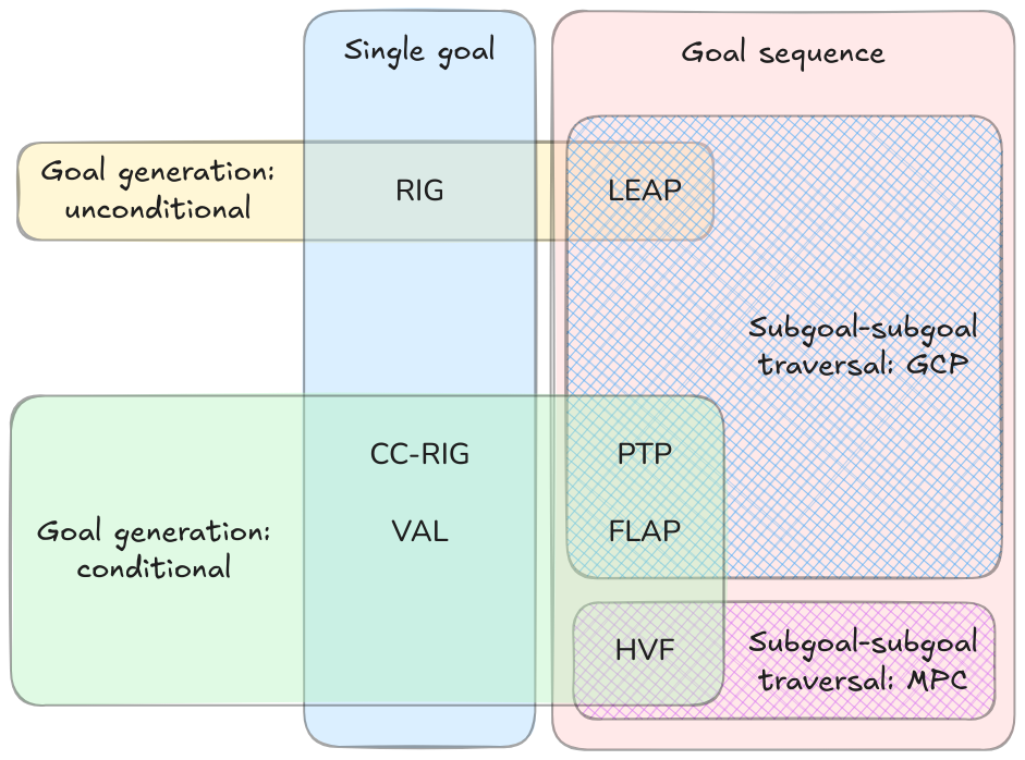
Back to themes

At the beginning I wrote that these papers basically explore four different “axes” of themes:

• Goal sampling: unconditional vs conditional sampling
• Goal generation: single goals vs subgoal sequences
• Subgoal feasibility: simple latent distance cost vs using the value function
• Method of traversing between subgoals: learned policy vs MPC

Now having gone over them above, we can draw out a Venn diagram type display of this:

Real robots is really impressive

If you’re not in the field, or you’re in the field but mostly do stuff on the computer, you might not know how big a deal it is to do stuff with real robots. The applications of RL are mostly “computational” at this point, with people applying it to areas like board games, video games (😉), LLMs, but it’s not yet widely applied to physical things. I’m sure that’s partly because it’s just generally less common to do any sort of physical experimentation, but RL is particularly weak in this area because it tends to be A) very “brittle”, and B) very data hungry, both of which make application to robotics really hard. That is, RL often doesn’t work well when it encounters the unexpected, and robotics is chock full of that (oh, the power cable is rubbing slightly more today, I guess I’ll die). In contrast, even really complex board games tend to be constrained to “behave” well. And (unless you’re going to do sim to real), collecting data with real robots is slow and expensive.

All this is to say that it’s really impressive! I think I recall hearing Sergey Levine saying somewhere that he applies his algos to robotics at least partly because it’s a true test of an algo working well.

The extent of my “robotics” experience is basically the dinky puckworld robot I made and trained in my basement, but it did leave a lasting impression on me. The difference between how long the “in simulation” part took to do (pretty quick) vs how long the real robot (weeks) took to get working still shook me. I was just learning about RL at the time and clearly (if you see the post) I was dealing with a bunch of dumb practical problems that actual roboticists wouldn’t get stuck on, but I think the specific problems change but the theme remains the same.

Extra thoughts on a few of them

• RIG:
  • Note that they train the VAE before the RL part (as opposed to at the same time). It’d probably be harder to train both simultaneously, but this means that you had also better hope that your original data distribution actually is expansive enough.
  • IIRC, they don’t do this here, but if you found that during the online RL part, you were discovering a lot of new data that you didn’t initially have when training the VAE, you can of course repeat the whole (train VAE, train RL) process multiple times.
  • Note that there are two kinds of similarity in the observations, and the form of the reward used above relies on them being similar enough: image similarity and temporal similarity. I.e., even though the images the VAE is trained on do come from trajectories, it has no info about that; when it embeds successive images from the same trajectory into (hopefully!) similar places in the latent space, that’s because they’re similar enough data that it makes sense to do that, in terms of the VAE objective. On the other hand, the RL models are optimized with sequences of observations from trajectories, and these do inherently have temporal information. The reward based on latent space distance only works because we (reasonably) assume that successive states might be different but not that different.
  • Note that although we train an encoder and decoder for the VAE, the decoder isn’t used at all after training. I.e., it’s simply used for training, and what we’re really after is a latent space with structure, corresponding to real states. This is in contrast to many common uses of VAEs, where the latent space is used to generate realistic samples in image space. This is a common theme in these GCRL papers, and in many you’ll see them do a different embedding paradigm where they do away with a decoder entirely.
  • Of their reasons for learning the VAE, I think the 2nd one is a bit silly, to be honest: plenty of RL methods directly learn from images. If you’re gonna use the structured transformation for something, then it makes sense, but that’s what their other two reasons basically are. It seems a bit redundant.
• FLAP:
  • “Kitchen sink” approaches can often feel like they’re just throwing a lot of different stuff at the wall and seeing what sticks. But, it does feel like at this point they had actually refined the ideas over the course of the previous papers and getting a good sense of what worked and what didn’t.

Other big “families”

This is a big family of GCRL methods I’ve read about, but there are some others that offer different interesting directions. Unsupervised Skill Discovery isn’t exactly doing what I’d call GCRL, but it rhymes enough that I think it’s worth going into.

Another that I think is really cool and seems to be getting popular in the past ~3 years is metric modeling methods. I briefly touched upon it last time when I discussed a few of the most common reward functions people use in GCRL, but the idea is that if you do GCRL with a reward function that’s just $-1$ every step until you reach the goal, the resulting GCVF ends up being (the negative of) a metric on states. Viewing it through this lens lets you do all sorts of neat things.