CCVAE experiments

In a few recent posts, we talked about Goal Conditioned RL (GCRL), doing a rough overview, some motivations for it, and some extra details and such about it. I followed this up with a niche-lit-review going over the “RIG family” of GCRL methods.

Today’s post is about some experiments I did towards solving a practical problem you might run into while doing GCRL. The ideas should be applicable to many GCRL methods, but I use some stuff from the RIG family as the base for it. I went over the backgrounds of that stuff in the RIG post, so check that out if you’re not familiar.

The high level problem I want to solve

The problem I’m trying to solve here is actually a very practical one that I quickly ran into when thinking about trying to use GCRL methods. It’s fairly agnostic to the type of GCRL method, so I’ll be using CC-RIG here, but it applies to most.

Let’s assume we have some environment, tons of data from it, and we’ve actually successfully trained our CCVAE model and the corresponding GCRL policy. Recall that this means that, for any state the agent is in, if you give me a goal state, we can plug it into the CCVAE, get the latent vector for the current and goal states, and plug that into the policy.

Neat! Now, the boss comes to you and says, “pretty cool CCVAE and policy you’ve trained on our environment! You’ve been talking a big game about how this model will be so good at solving downstream tasks without having to redo the whole RL training process over, so I’m hoping you can help us. Here are 1000 example trajectories where we know a certain type of goal was achieved at the end of them. I want you to use your fancy models to give us a policy that can achieve that same type of goal, but from any state it finds itself in.”

Oh no, you think. Oh god. I thought we were just goofing when we talked about “applications”… I didn’t think they’d actually expect me to use this thing! So, how are you gonna do it?

Approaches

A simple approach…

Naively, this doesn’t seem so bad. In many cases, if your observation space was relatively simple, in terms of state variables, you might be able to just do a bit of analysis and see what part of the state vector defines the goals. Then, for any given state the agent finds itself in, you just take that state and modify the part of the state vector to make it equal to value for that goal, and use this modified state as the goal. You plug it along with the state into the policy, and the policy should go to the goal.

For example, let’s say the env is a simple 2D gridworld, and the observation is just a vector of the value of what’s inside each grid cell, $c_{i, j}$, for the cell at coordinates $(i, j)$.

\[s = [c_{0, 0}, c_{1, 0}, \dots, c_{n, 0}, c_{0, 1}, c_{0, 2}, \dots, c_{n, n}]\]

So, you look at a few of the “achieved goal” trajectories, and notice that the goal is always the agent going to the closest corner cell to its current position. Therefore, for any possible state the agent is in, you could just do a bit of “surgery”: find the agent’s current position, calculate the closest corner to it, and then make the cell for the current position empty, and mark the goal position cell as having the agent in it. So if the agent was in cell $(1, 2)$, the closest corner is cell $(0, 0)$, so for the state vector $s$ we’d create the goal vector $g$ by setting $c_{1, 2}$ to be “empty” and setting $c_{0, 0}$ to be “agent”, and leaving all the other entries the same. Sounds good, problem solved!

…which probably won’t work

For very simple problems, this might work. But it probably won’t work for more complex problems, even for state space observations: in many cases, the goal will be more complex than a single, easily identifiable part of the state. Similarly, even if it actually can be specified by a single part of the state taking on some value, it might involve many other parts of the state changing in unpredictable ways.

For example, let’s take the example above, but now there’s a slight twist: the ground of this 2D gridworld is covered in snow, such that when the agent moves anywhere, it melts the snow in that cell. This means that if it moves to a cell, there will necessarily be a “trail” of the cells it visited along the way to that cell. Now, if we try to do the “surgery” method above, we can’t just change the value of the agent’s current cell and the value of the target cell. This wouldn’t be a valid goal state from the current cell, because there’s no trail of melted snow from the current to the goal state.

Maybe you could make a function to solve for a plausible melt trail. Or, maybe it just doesn’t matter and plugging in the goal state with no trail would work fine. But this is a really simple example and you can easily imagine the concept extending to cases that aren’t easy to come up with, or where the implausibility of the state would matter a lot!

But it still gets worse. At this point, the general problem any “real” method should be trying to solve is learning from images. And with images, no approach like this can possibly work; in general there’s no “part” of the image that corresponds to a goal, there’s just some semantic meaning in there. So going forward, we should be picturing images for the observations.

This is the real problem: we have some examples of the goal, but they’re high dimensional, and for any given new observation (image), we have no straightforward way of producing the corresponding goal (image).

It’s worth saying that this problem isn’t specific to CC-RIG. Most GCRL methods work by embedding the observation into a latent space, and having the models take inputs from that latent space. I’m just using CC-RIG here because it’s relatively easy to get working.

The high level strategy

The high level strategy I’m considering here is searching for the goal in the latent space. The key idea is that we’re using a latent space in the first place because the original space is too high dimensional and unstructured, but the latent space is much smaller and should capture the meaningful parts of the environment.

From a high level, we can formulate the problem and approach this way:

• We have some massive dataset of pairs of states, where in each pair the second state is one that could follow (not necessarily immediately) the first state, in our environment: $\mathcal D = { (s_i, s_{i+1}) }_i$
• Using, $\mathcal D$, we learn:
  • some sort of embedding $\phi$ that embeds states into a latent space: $z = \phi(s)$
  • a GC policy (and other models) that have been trained on and operate on this latent space: $\pi(z, z_g)$
• After that training, we’re given another, much smaller dataset of pairs of states for a given goal type, where in each pair, the second state is the goal state from the first state, and whose distribution is a subset of $\mathcal D$: $\mathcal D_g = { (s_i, g_i) }_i$
• Now, for any raw state $s$ (which we can already calculate the latent for, $z = \phi(s)$), we want to find the corresponding $z_g$ to plug into the policy to go to that state
• Therefore, we want to use $\mathcal D_g$ to produce some sort of process $f$ that does this mapping: $f: s \mapsto z_g$

There are a variety of ways we could try. Today I’ll just try the simplest, to see how it fares, and in the future I’ll try others.

I also won’t actually be doing the RL part here – we’re assuming the policy can go to any given legitimate goal, so this post is really more about just producing the legitimate goal.

The toy env

At this point it’ll be useful to get concrete and show the toy env I’ll be using, so I can use it to illustrate examples. It really is a toy env (and therefore doesn’t really have the pitfalls “real” problems have), but it has enough to show the ideas.

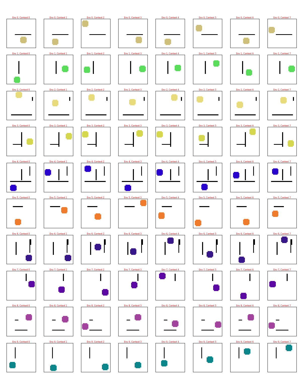
This toy env is from the CC-RIG paper. The environment consists of a 2D grid of pixels, with walls colored in black and a circle (representing the agent) colored with a value in some lightness and saturation range so it’ll be reasonably distinct from the background and walls.

Importantly, each “episode” we sample a new “env”, i.e., a set of 0-3 horizontal and vertical walls, and a color for the circle in the episode. I say “episode”, because as I mentioned above, we’re not actually doing any RL here, but the point is that the agent would experience a distribution of these envs over different episodes, which is the distribution we’re trying to model with the CCVAE. For a given “episode”, the wall positions and circle color are fixed, but the different possible states for that episode could have the circle in any position that doesn’t have it intersecting the walls, and fully inside the grid.

Here are some random examples, where each row is a sampled “env”, and each column in that row is a state from that env:

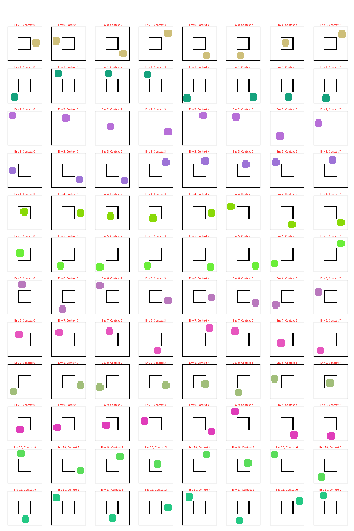
I’m going to informally say “env” to mean a sampled environment, i.e., a given position of the walls and circle color. Note that for a given env, the circle color and wall positions are the same, but the circle moves to different valid positions.

Types of goals

Our assumption is that the CCVAE and policy have already been trained on a ton of data, so for any type of goals the boss might come to you with, the models may not have seen literally those specific goals, but we have enough data coverage that it has definitely seen that type of goals.

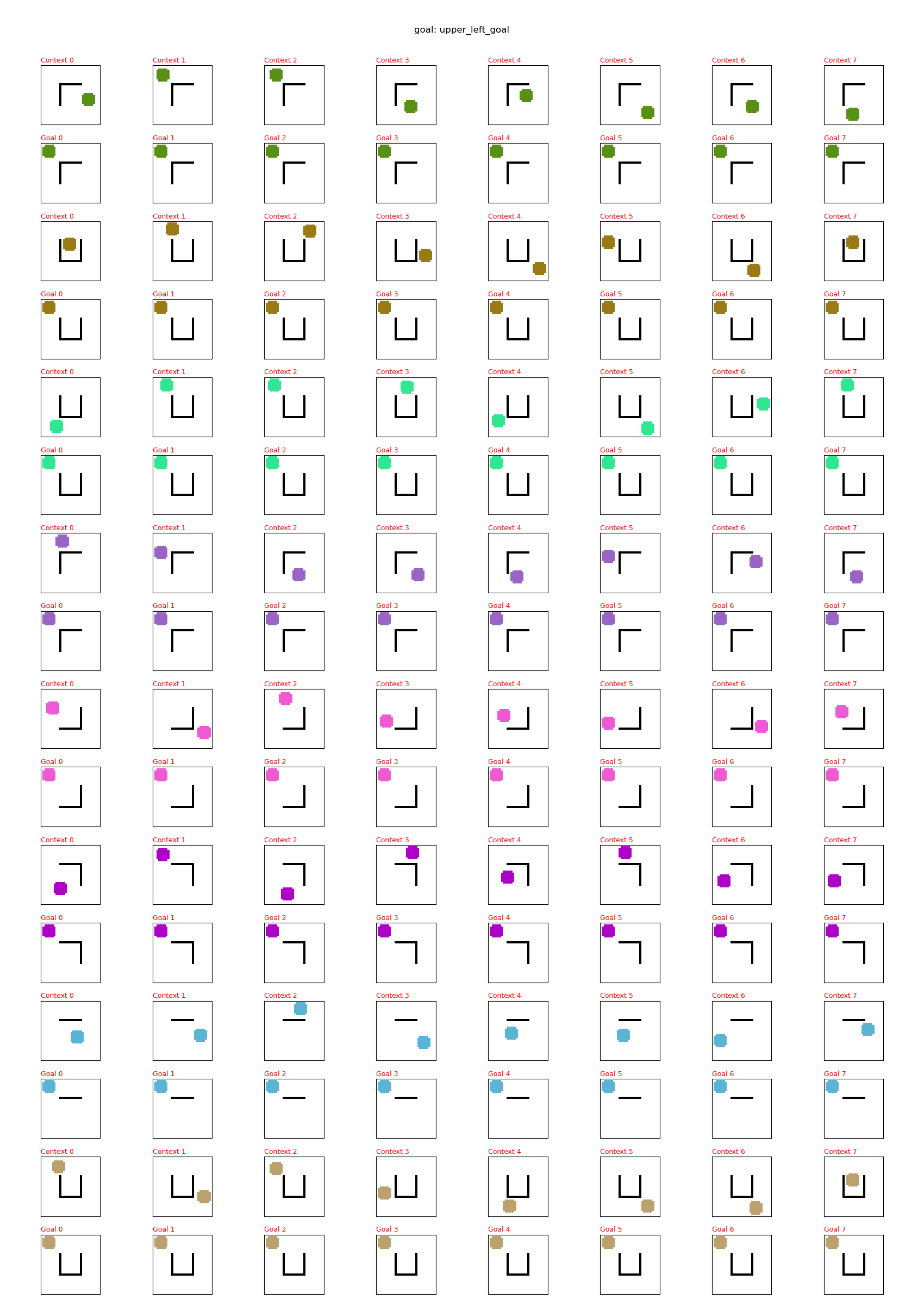
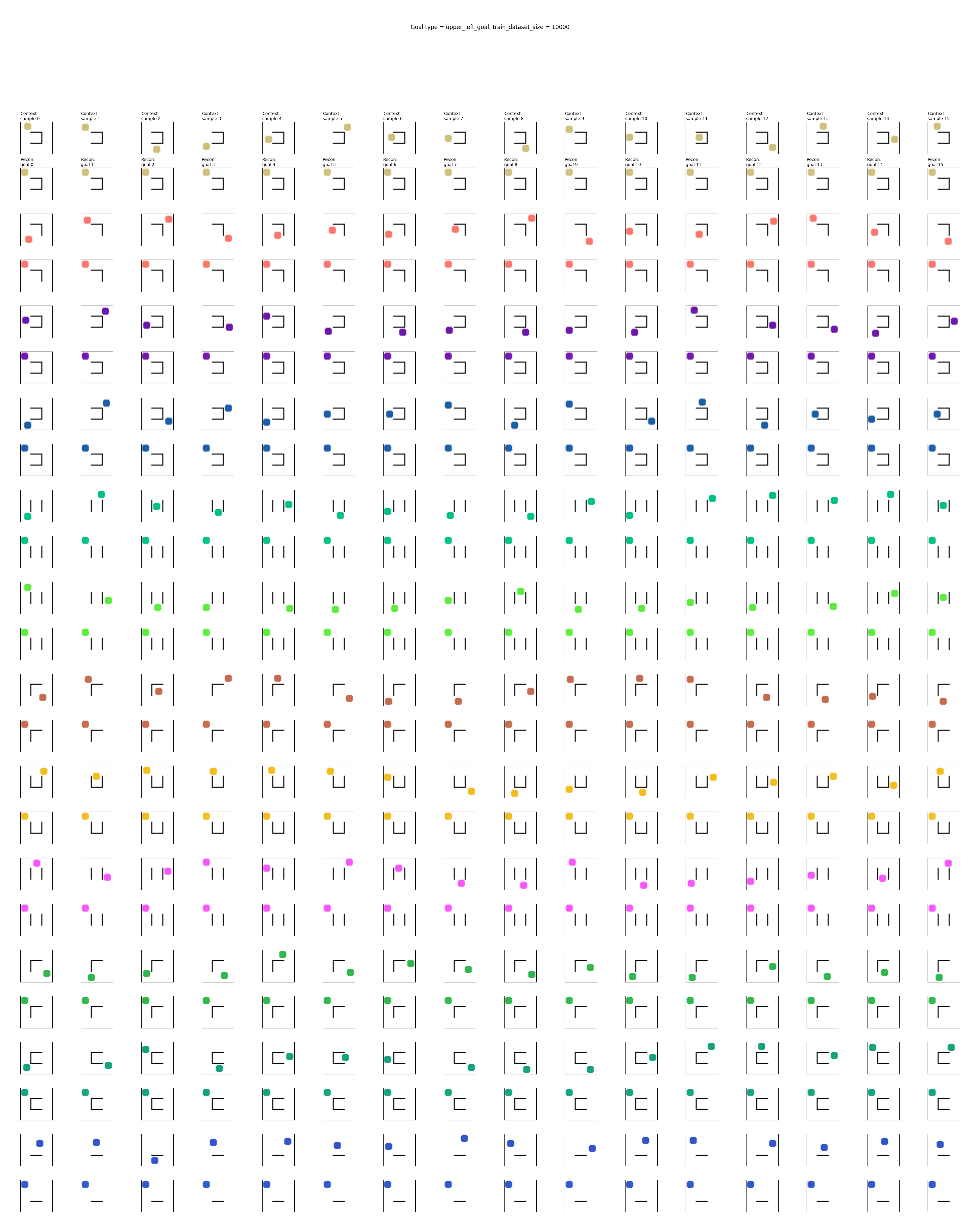
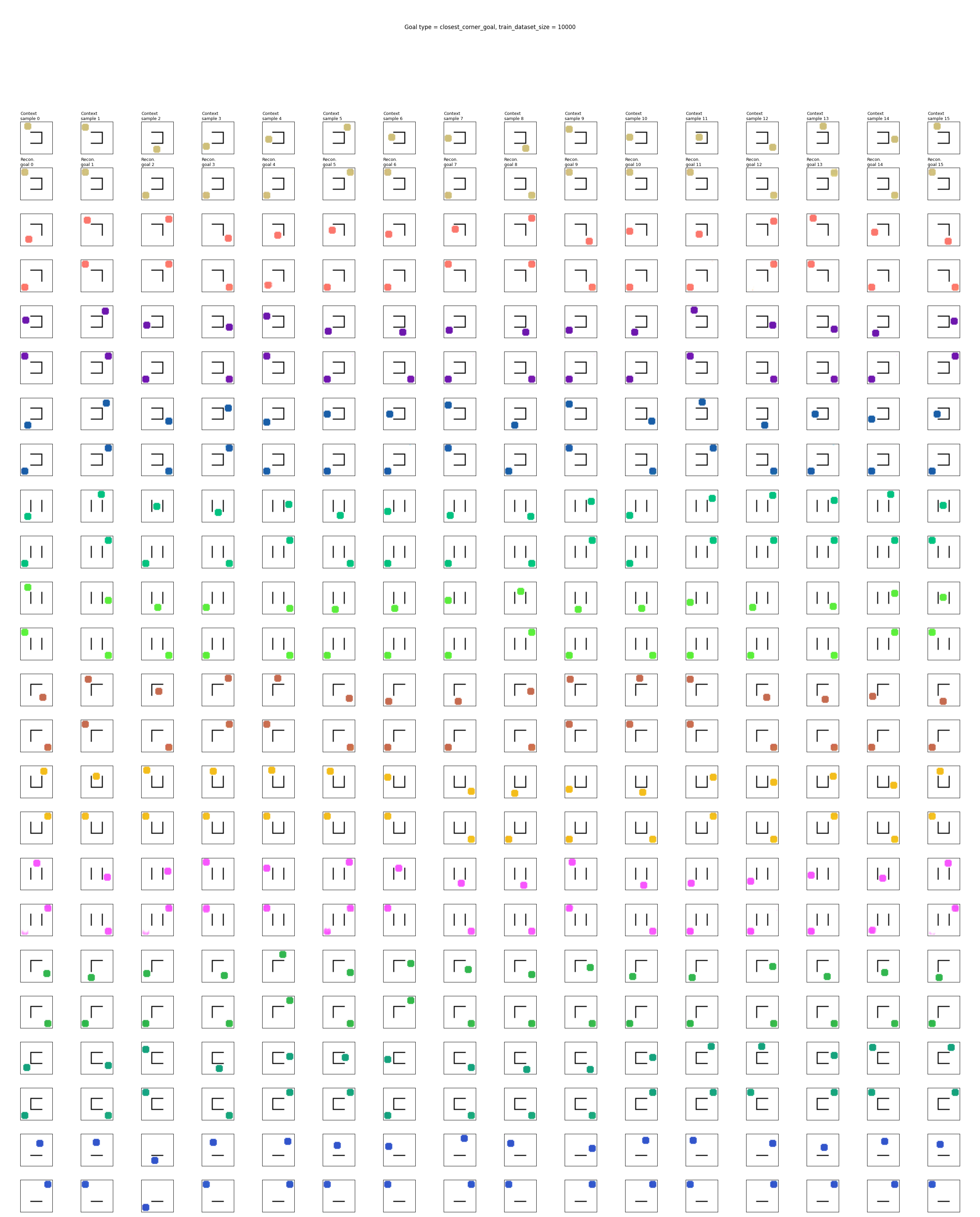
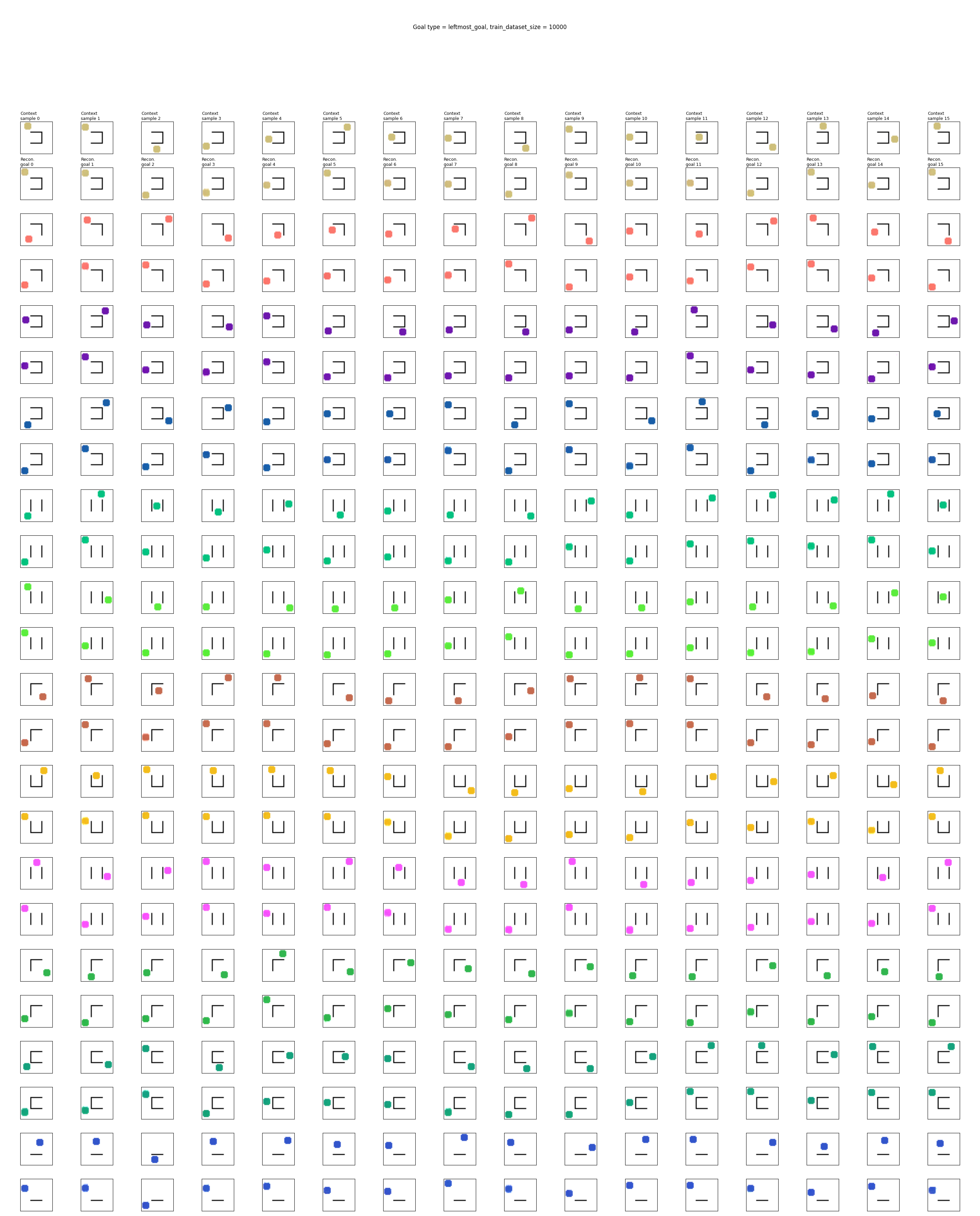
Here, I want a few different types of goals, to test various difficulties. In the plots below, there’s a pair of rows for each env (for example, rows 1 and 2 are for env 1, rows 3 and 4 are for env 2, etc). It should hopefully be clear because the pair of rows will have the same color circles.

In each pair of rows, each column of the top row is a sampled state from that env, and the column in the bottom row is the corresponding goal for the sampled state.

Static “upper left corner” goal

The simplest goal is “circle moving to the upper left corner”. This is obviously very very simple, but note that it still does depend on the context: for the goal, the circle must be the same color, and the walls must be in the same positions (i.e., the same sampled env).

However, it’s obviously very simple, in the sense that for a given env, all the valid states for it have the same exact goal state. So it’s really just a sanity check to make sure it can learn the broader context.

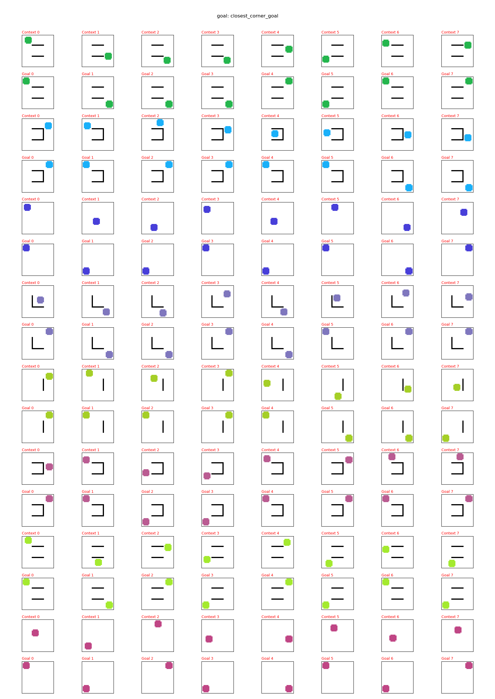
Closest corner goal

This one is slightly harder. It moves any state to the closest corner, as far as it can get to that corner without intersecting any wall. So, the goals won’t be the same for all states of an env. Still, for a given context, there are only 4 possible goals.

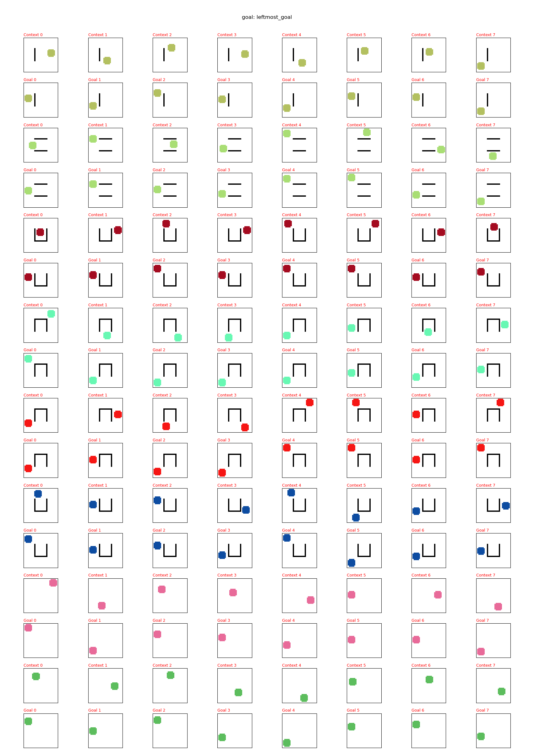
Move as far left as possible

For this goal type, for a given state, the goal is the farthest left state that’s at the same height and not intersecting a wall.

Goal proposal model

Like I said, today I’m gonna do a real dumb one. This post is already getting long winded from laying out the background, so I’ll try some other ideas in a future post.

The main idea is this: to produce the mapping $f: s \mapsto z_g$, we’ll directly train a plain old feedforward NN that learns to map the latent vector $z$ to the latent goal $z_g$. I.e., for each $(s, g) \in \mathcal D_g$, we apply $\phi$ to get $(z, z_g)$, and then train $f$ to minimize the loss $|z_g - f(z)|^2$. Then, to use it in a given state $s$, we can calculate $z_g = f(\phi(s))$, and plug that into the policy.

Note that, like I mentioned above, this approach should be general to any method that’s embedding the state to a latent and using a policy that operates on the latent space, which encompasses the majority of GCRL methods. So the block diagram of this vague thing would be:

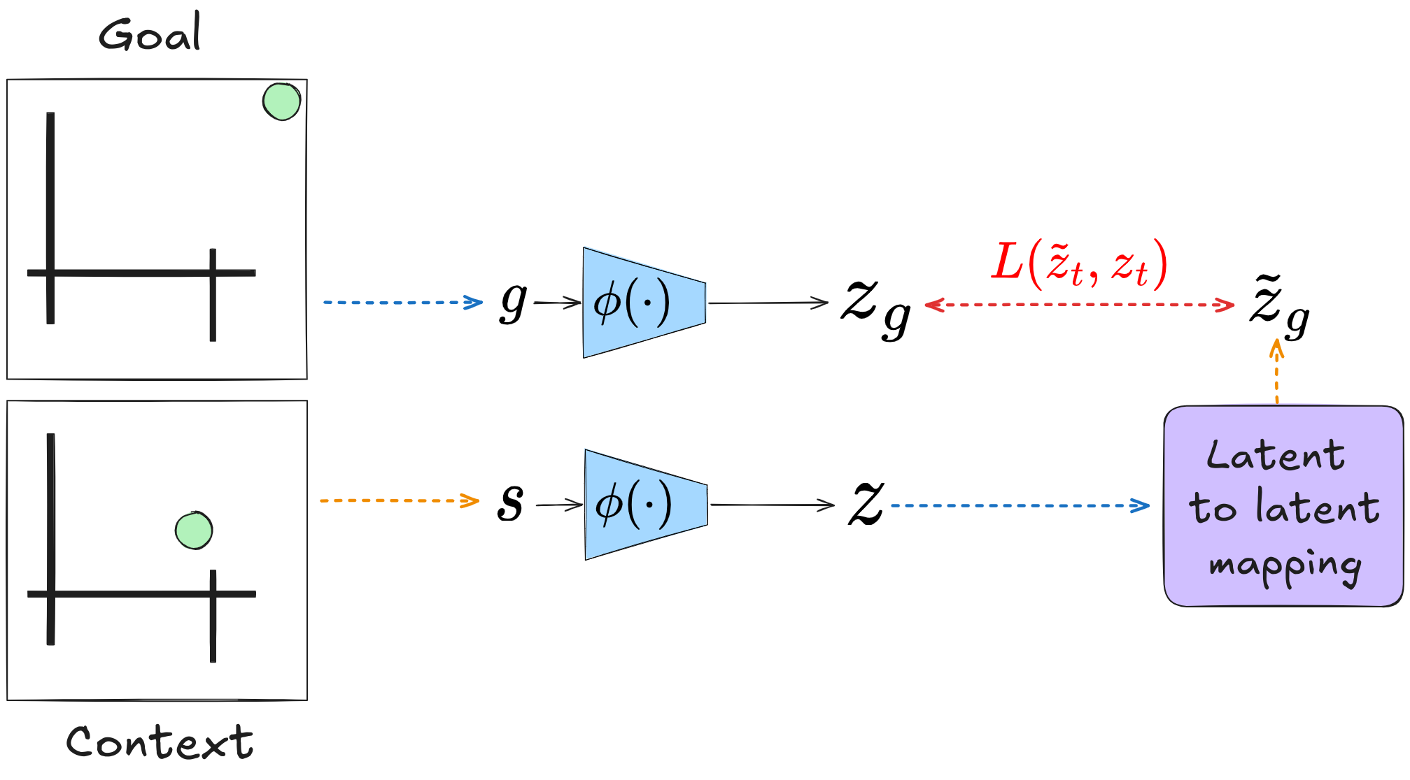
Hey, I warned you it was dumb! I’m just seeing how a naive approach works, first.

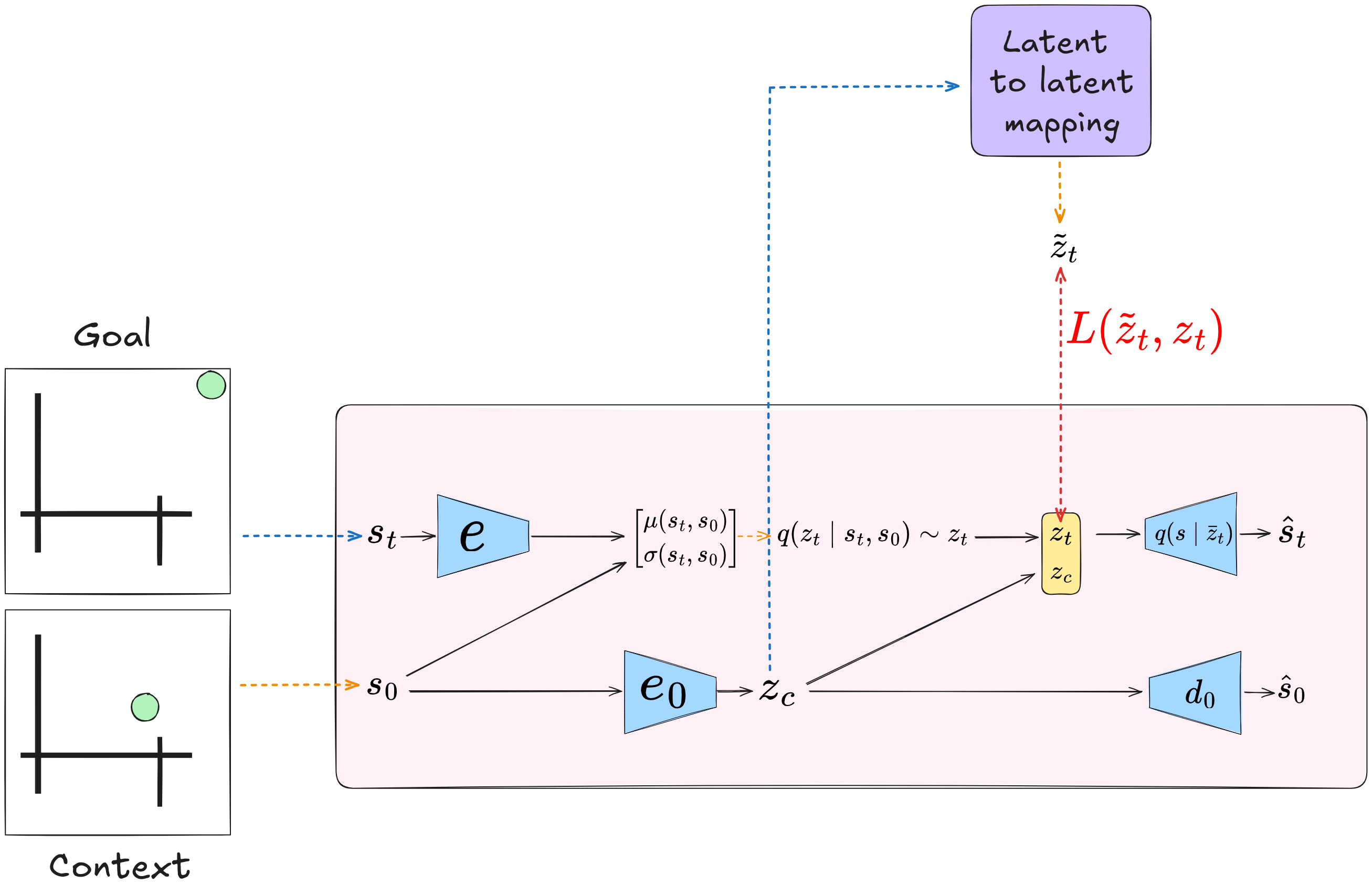
In the specific case of CC-VAE, the approach should actually be a bit easier, for the following reason: we form the (full) latent from the latent context and the other latent part. The whole point of using the CC-VAE is that most of the “burden” of reconstructing the state falls on the latent context, which can be a larger latent space and doesn’t have the information bottleneck, while the latent component that is responsible for the distribution of states from that context can be much smaller.

This means that for the CC-VAE, we don’t have to map $z$ to the “full” $z_g$, we only have to map it to the small “latent feature” part ($z_t$) that “modifies” $z$ ! Let’s call this approach “latent to latent mapping”. The block diagram would look like:

Experiments and results

CC-VAE results

First, let’s just look at how the CC-VAE does, since the rest will be downstream from that.

Below are the reconstructions of features for a given context, where the leftmost column shows the context for the env, and each env has a pair of rows. The top row are real data samples for that env, and the bottom row are those ones reconstructed from the context and top row:

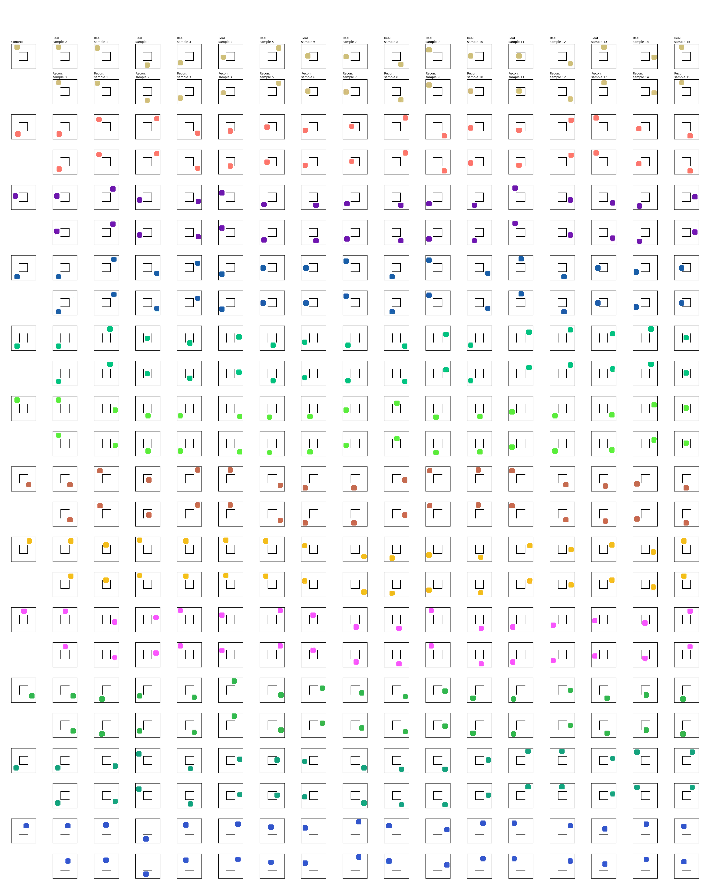
This tells us how well it can reconstruct the real samples from the context and their values in the latent space. This is usually pretty easy, as you can see.

Next, let’s look at some samples from a given context, reconstructed so we can see what they look like in image space. If everything is learned well, these should all look like real samples from that env. Below, the 1st column is the env with no circle, the 2nd column is the context used for generating samples from that env, and the following columns are using that context, sampling a latent feature value, and decoding it to create a sample. Here’s an example of that:

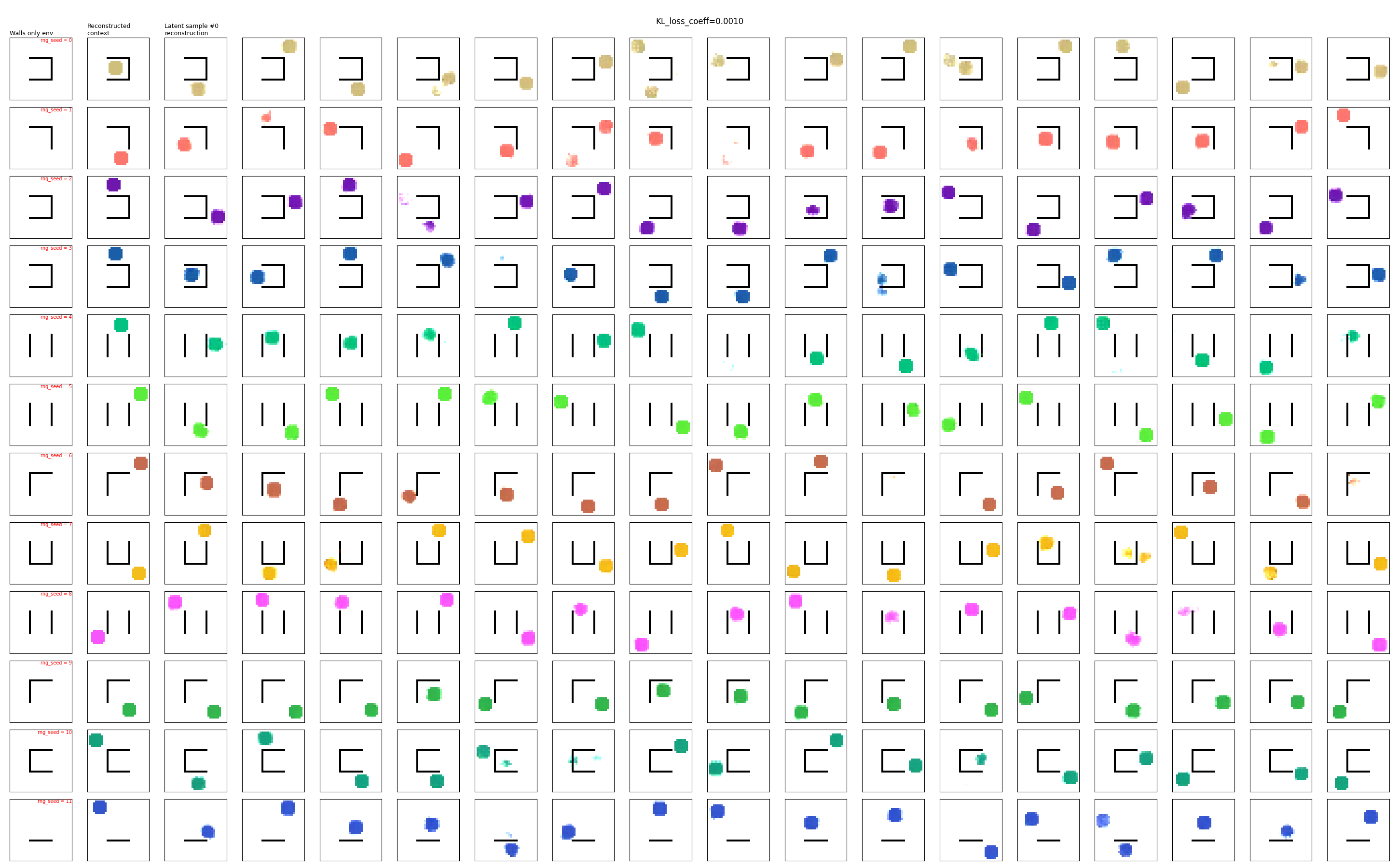
You can see that they’re mostly pretty good, and the majority look like real samples. However, there are a minority where 1) the circle is missing, or 2) the circle is there but messed up, or 3) there are two circles. More on this later.

One last thing we can look at is the latent space itself. I’m using a 2D latent space here, for a few reasons:

• Most of the state information should be contained within the latent context (which is not constrained by any info bottleneck), meaning that the latent feature part can be very small
• The latent dimension is a double edged sword: larger dimension means that it can more easily encode and reconstruct, but it also means that unless the encoded data is actually filling the latent space well, large regions of the latent space will correspond to no real data. In that case, when you sample from the prior, you’ll get lots of unrealistic garbage reconstructions. In our case, we really want the latent space to have as much meaningful structure as possible, so we want to make sure the data fills it effectively (while still being able to reconstruct obviously), meaning that smaller is probably better
• Conditioned on a given env, the state is defined only by the position of the circle – which is basically a 2D number, so a 2D latent makes sense
• and of course, being able to visualize is always handy and looks cool :P

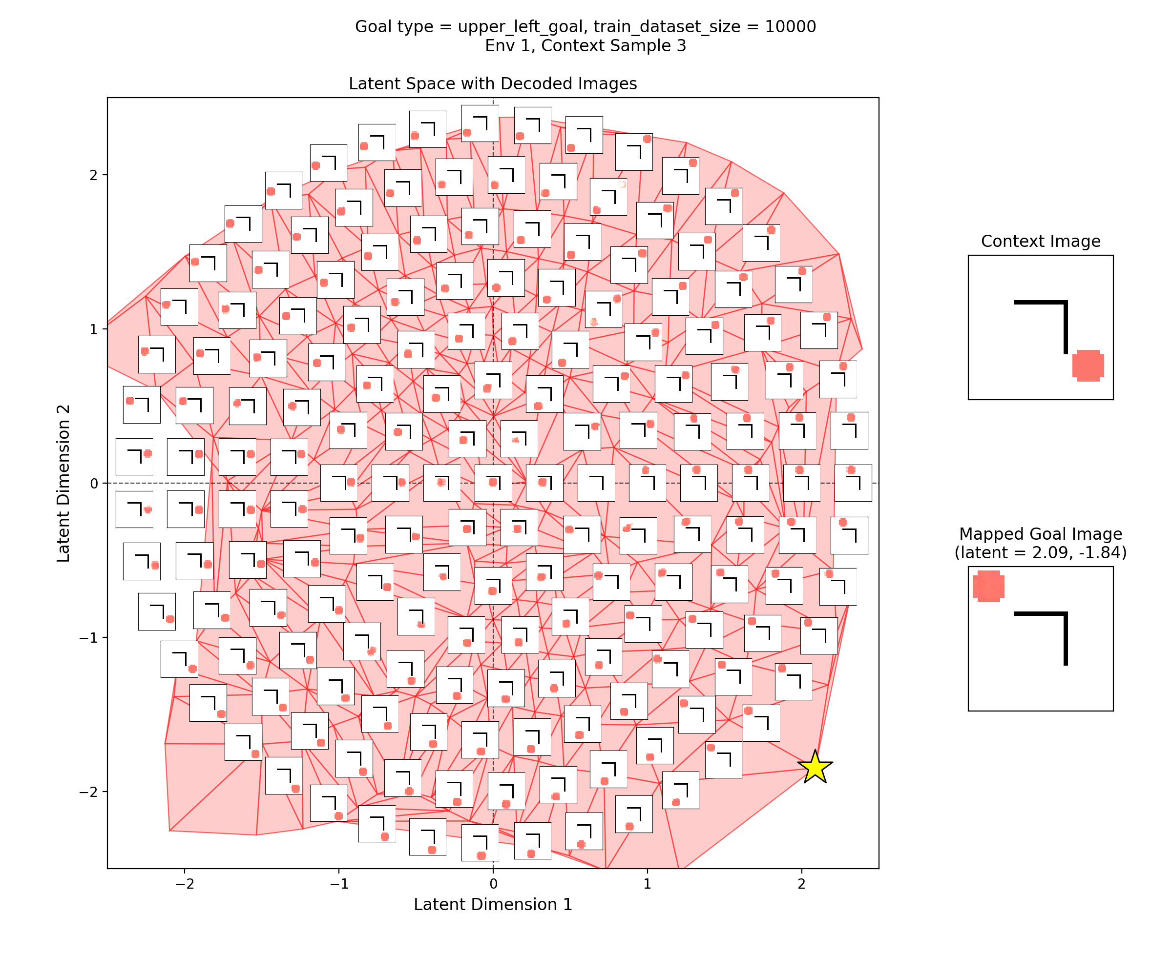
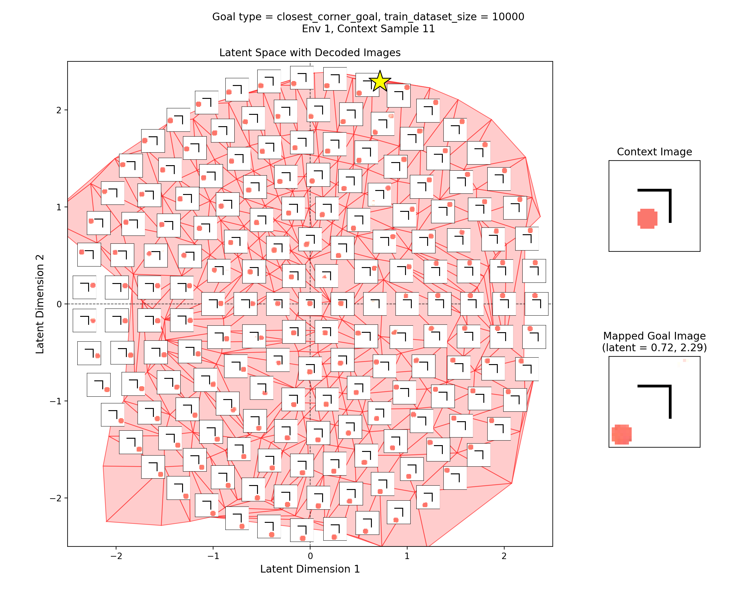
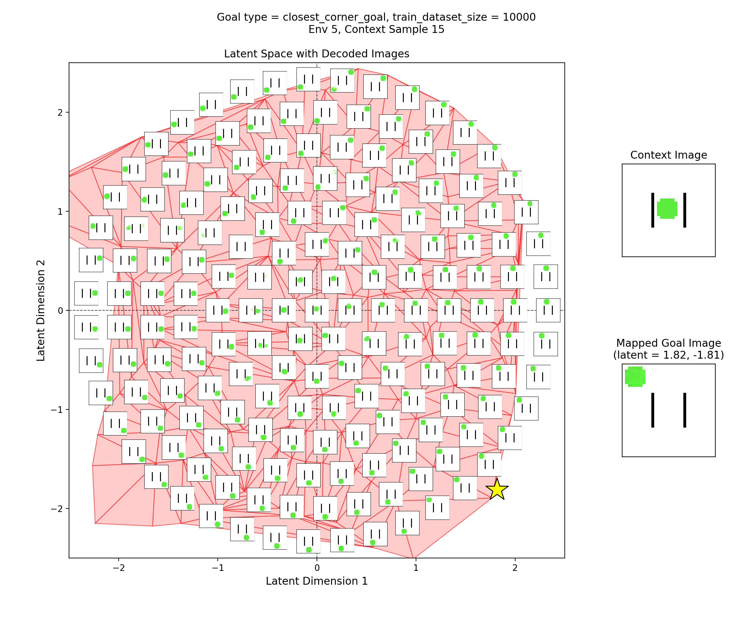
To visualize the latent space, I made plots like this:

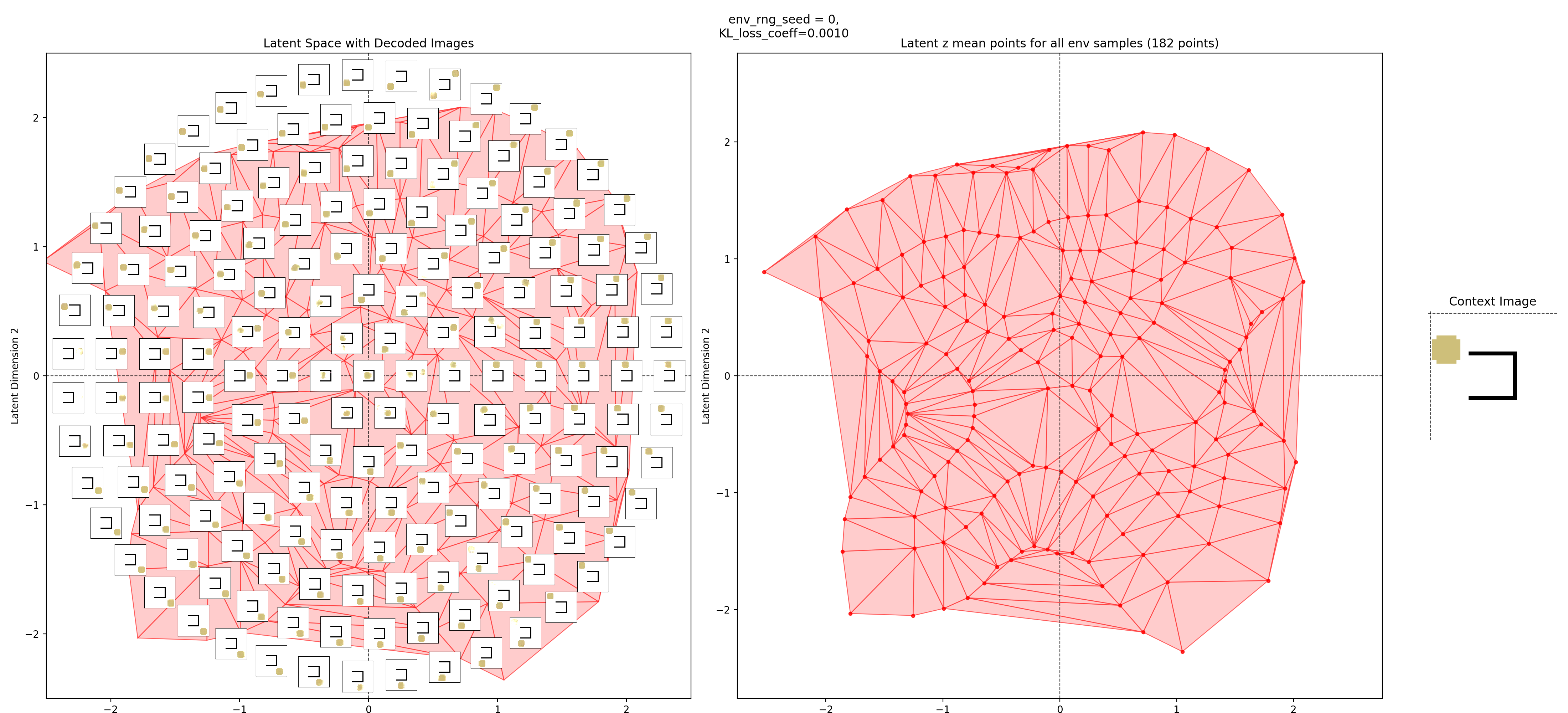
In the left subplot, I’ve taken a bunch of 2D points of the latent space, and using the context shown in the right plot, decoded them to show what those latent points get reconstructed as (inset at each of the latent points). I used a few concentric rings out to a radius of a few standard deviations, which should cover ~95% of the standard normal prior is two dimensions.

In the middle plot, I’ve taken all the real state images for that env and encoded them into the latent space, using the same context. Each red point in that plot is one of the real datapoints (images). Since there aren’t many of them (100-300 usually), I’ve done a Delaunay triangulation with some tidying to better visualize the “area” the encoded real data covers. I’ve then taken this triangulation and plotted it in the background of the left plot.

Together, these were actually pretty helpful for diagnosing and debugging stuff. They can tell you if your encoded data isn’t matching the prior well, if the triangulation doesn’t cover most of the region with the insets. If there’s a region of the latent space where the encoded data is there, but the reconstructed inset images don’t look good, that implies that the decoder is probably messed up.

Latent mapping results

Okay, so how does the actual latent mapping do?

Goal types

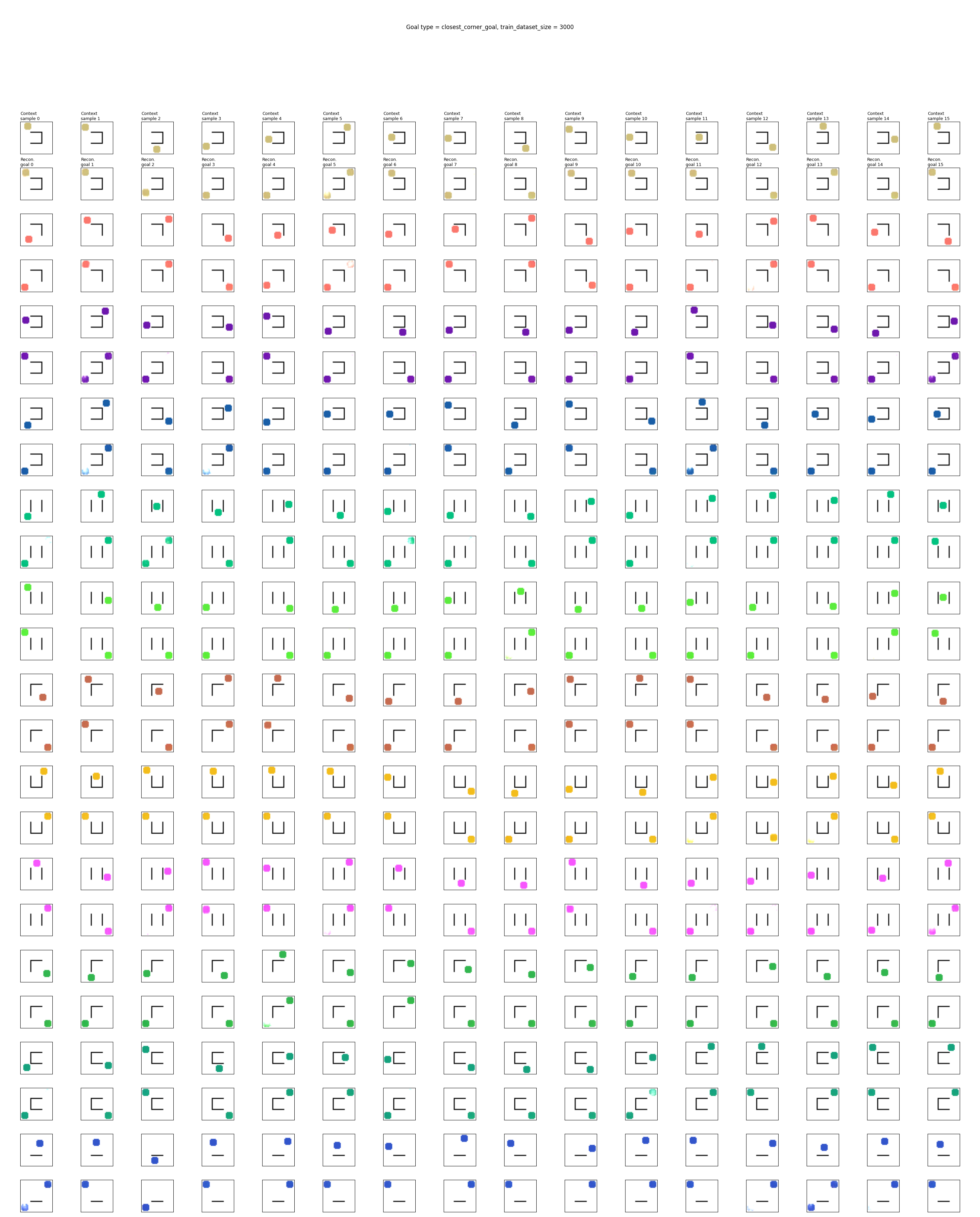
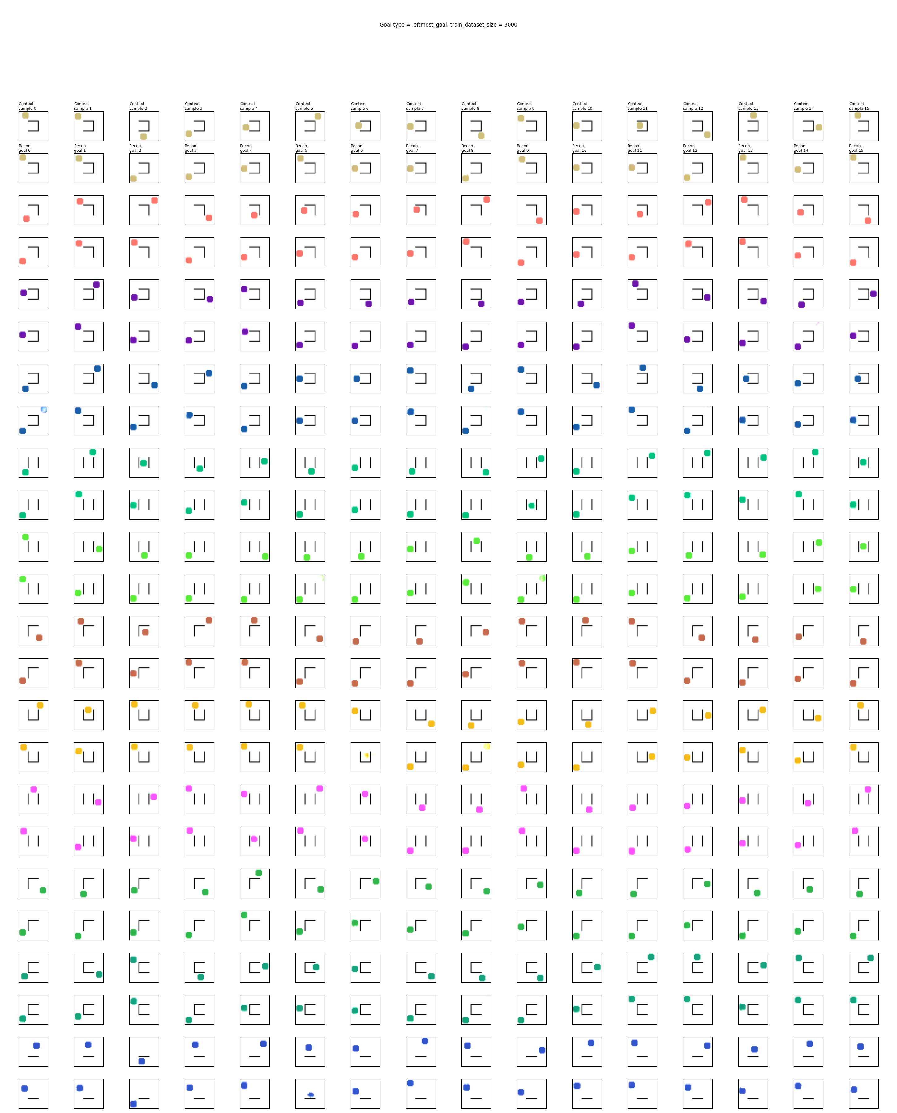
For each of the goal type mentioned above, I’ll show a large grid with pairs of rows, where the top row in the pair is the “context” or “current state”, and the bottom row is the goal that the latent mapping produced, decoded to give an image. This will let us quickly see if it’s broadly succeeding for the goal type across multiple envs.

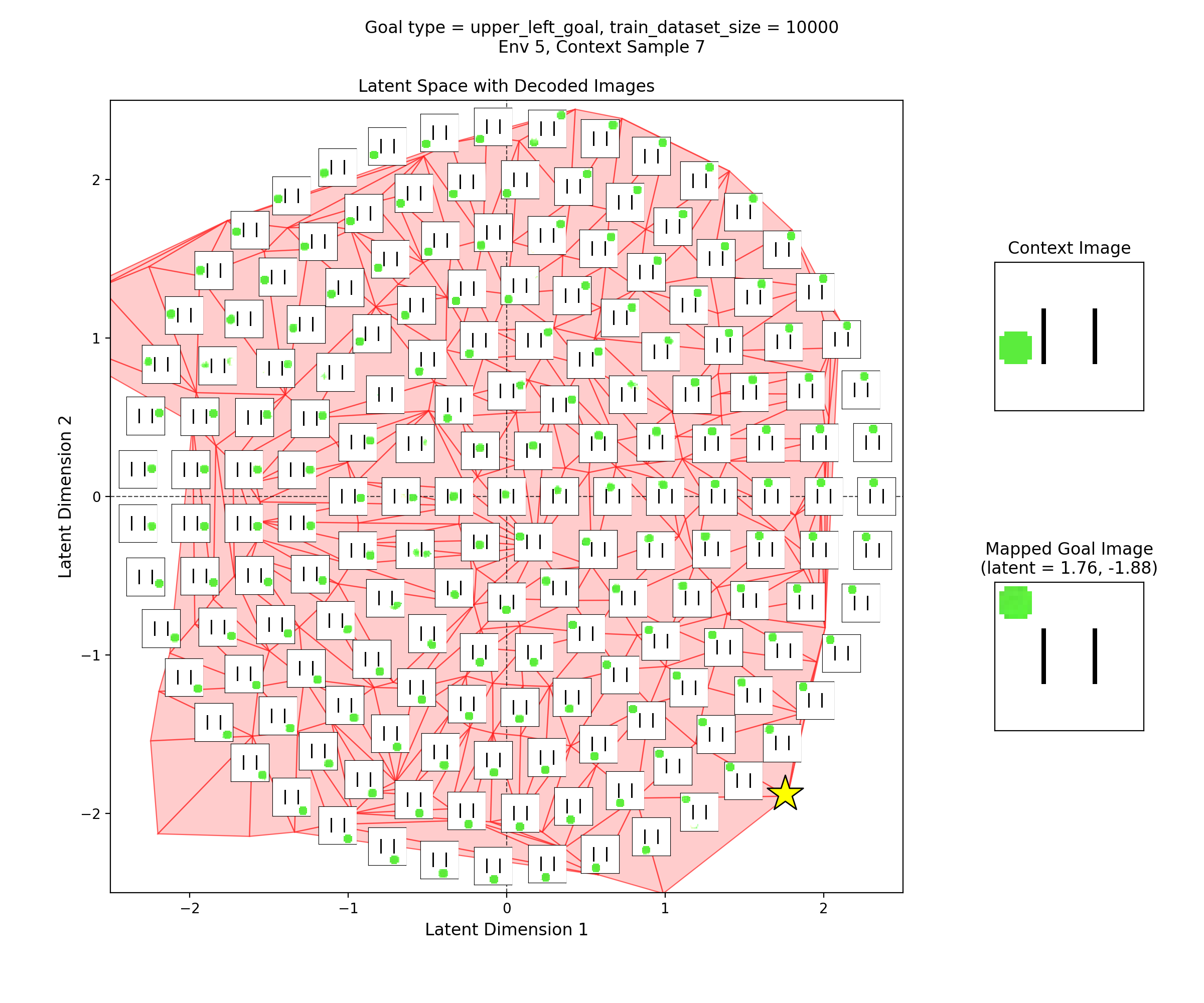
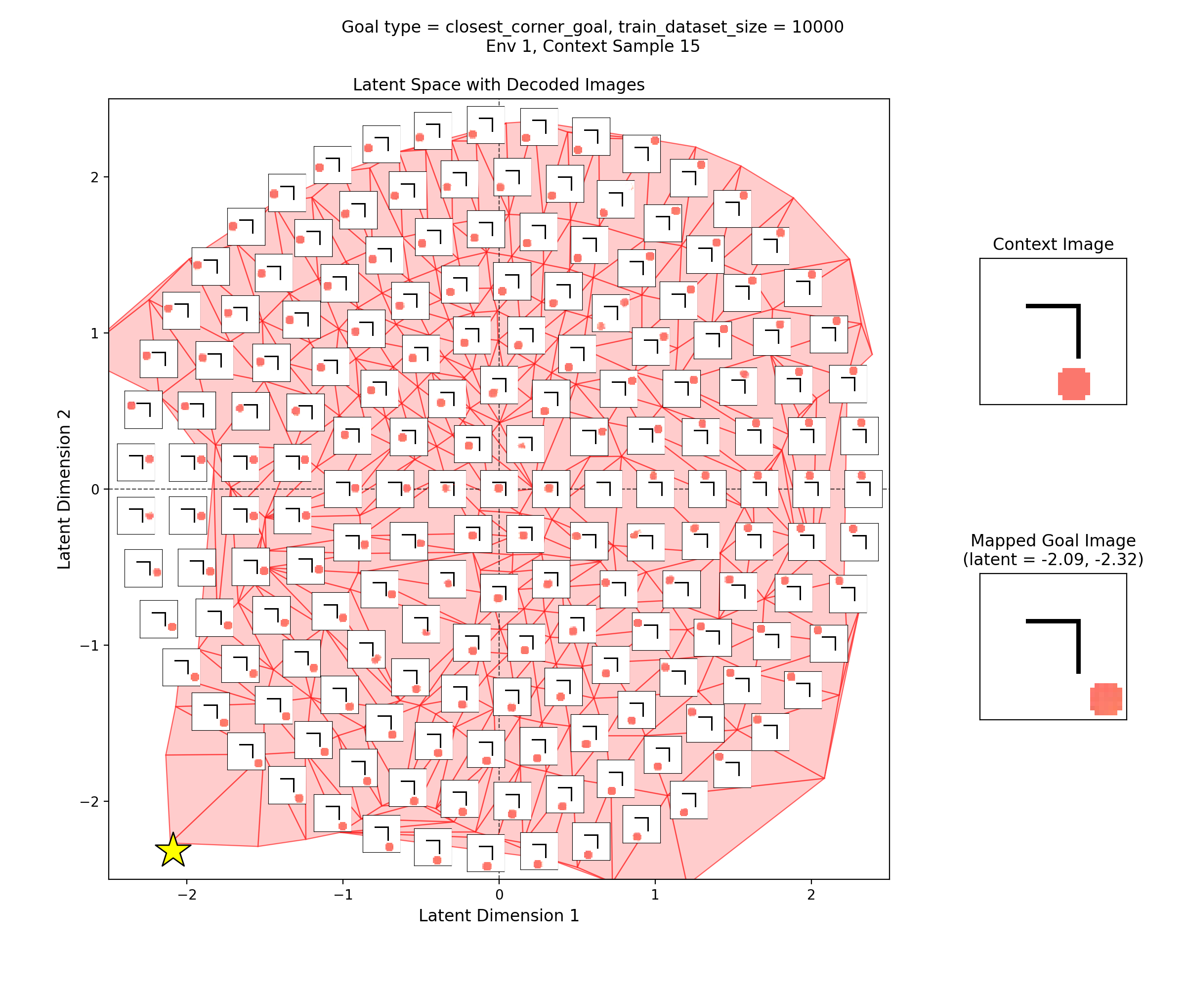
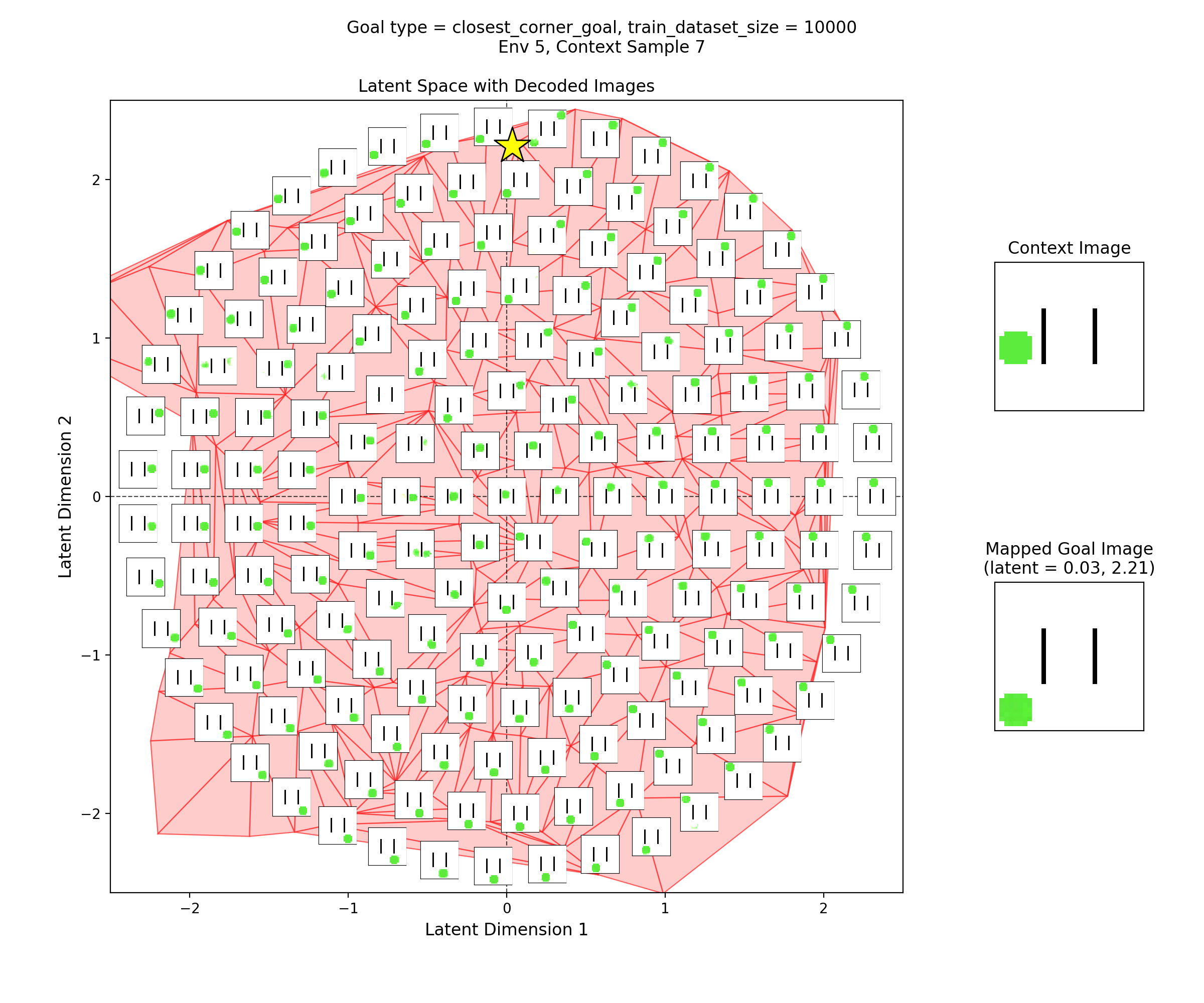
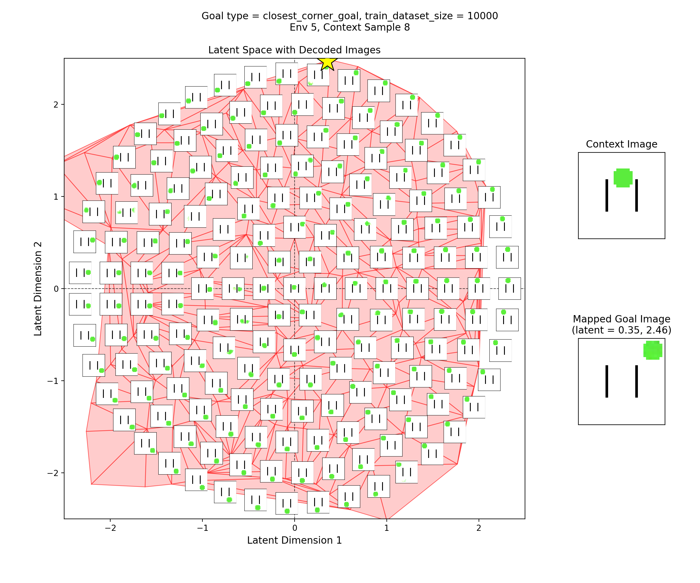
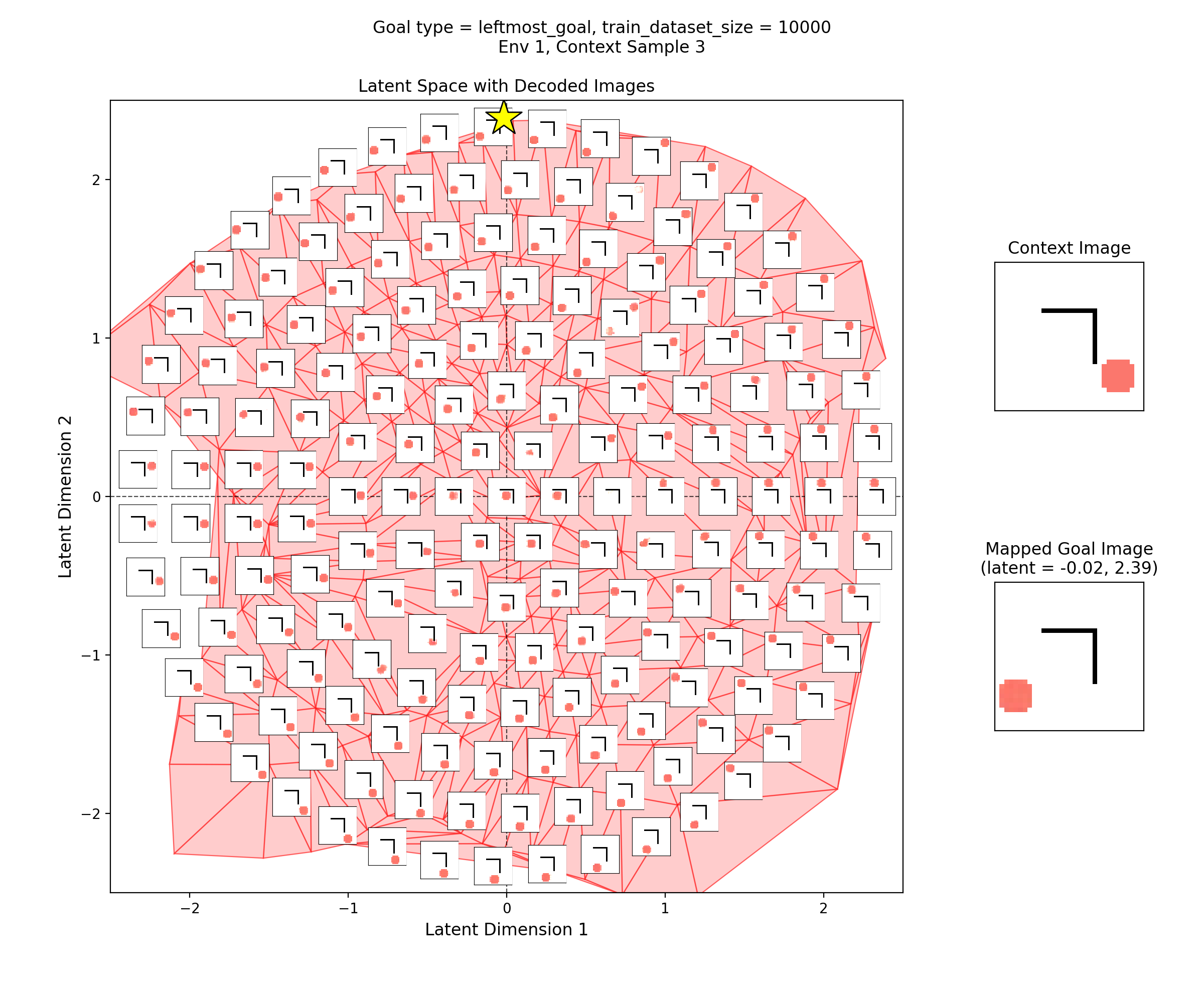
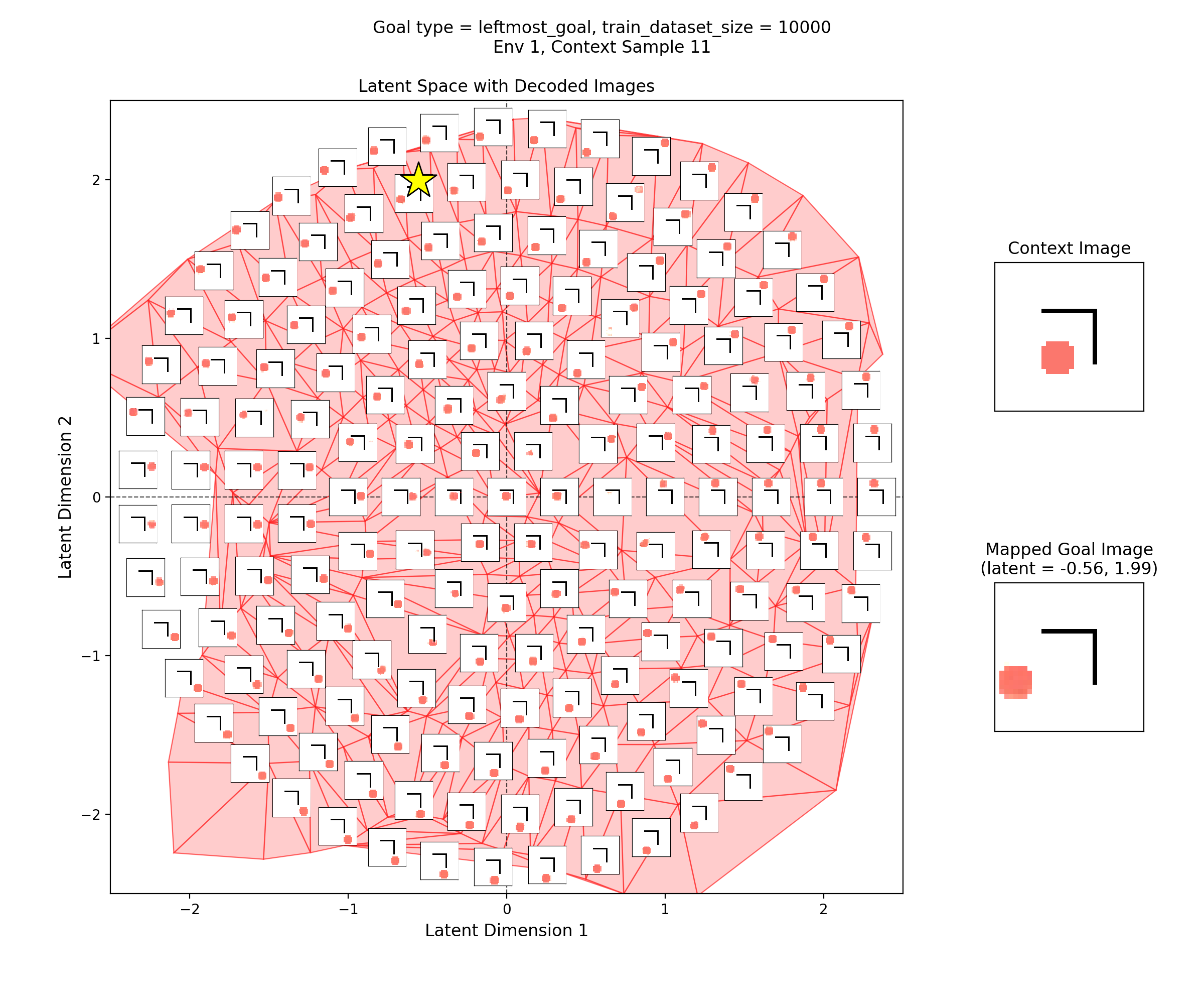
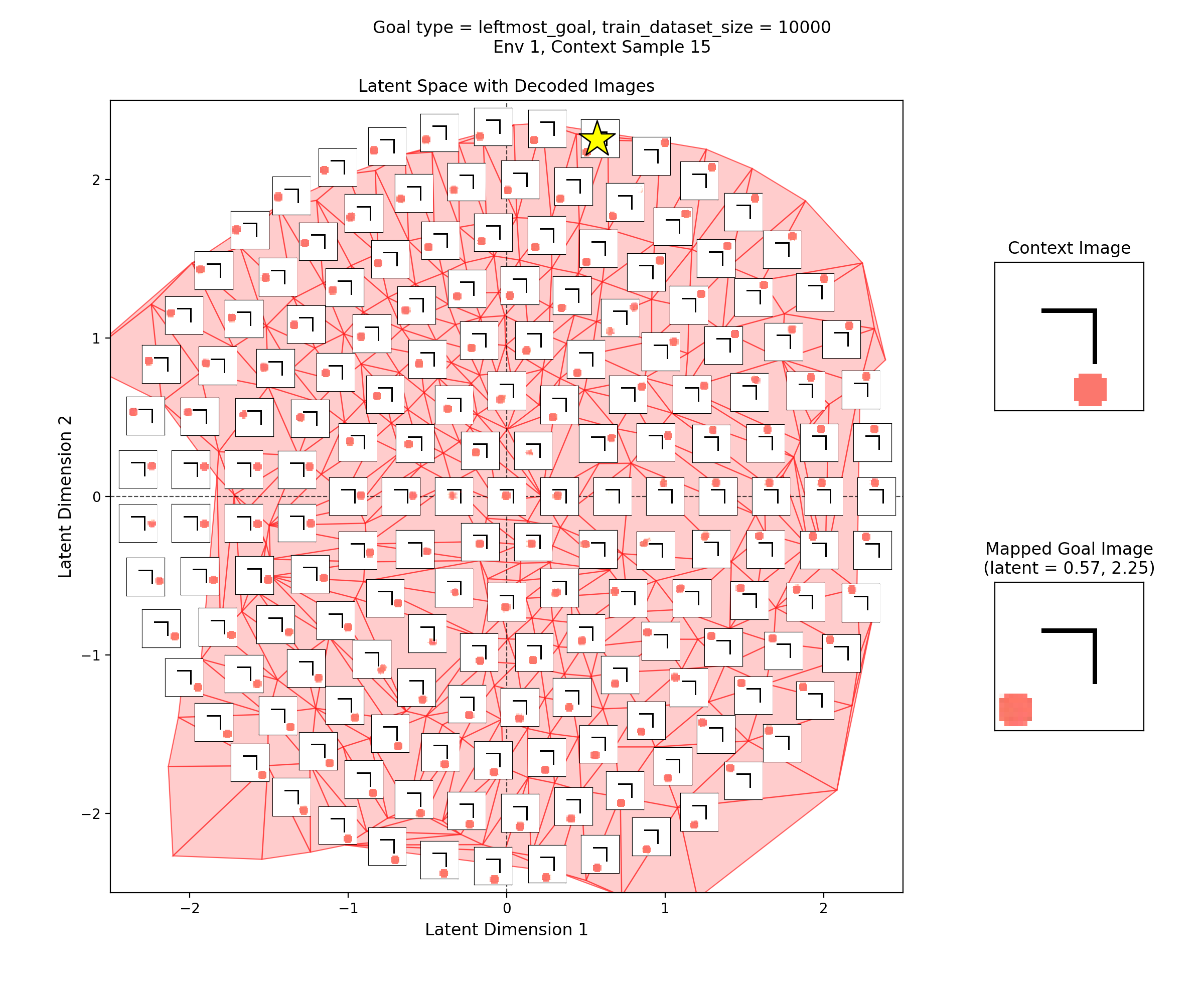
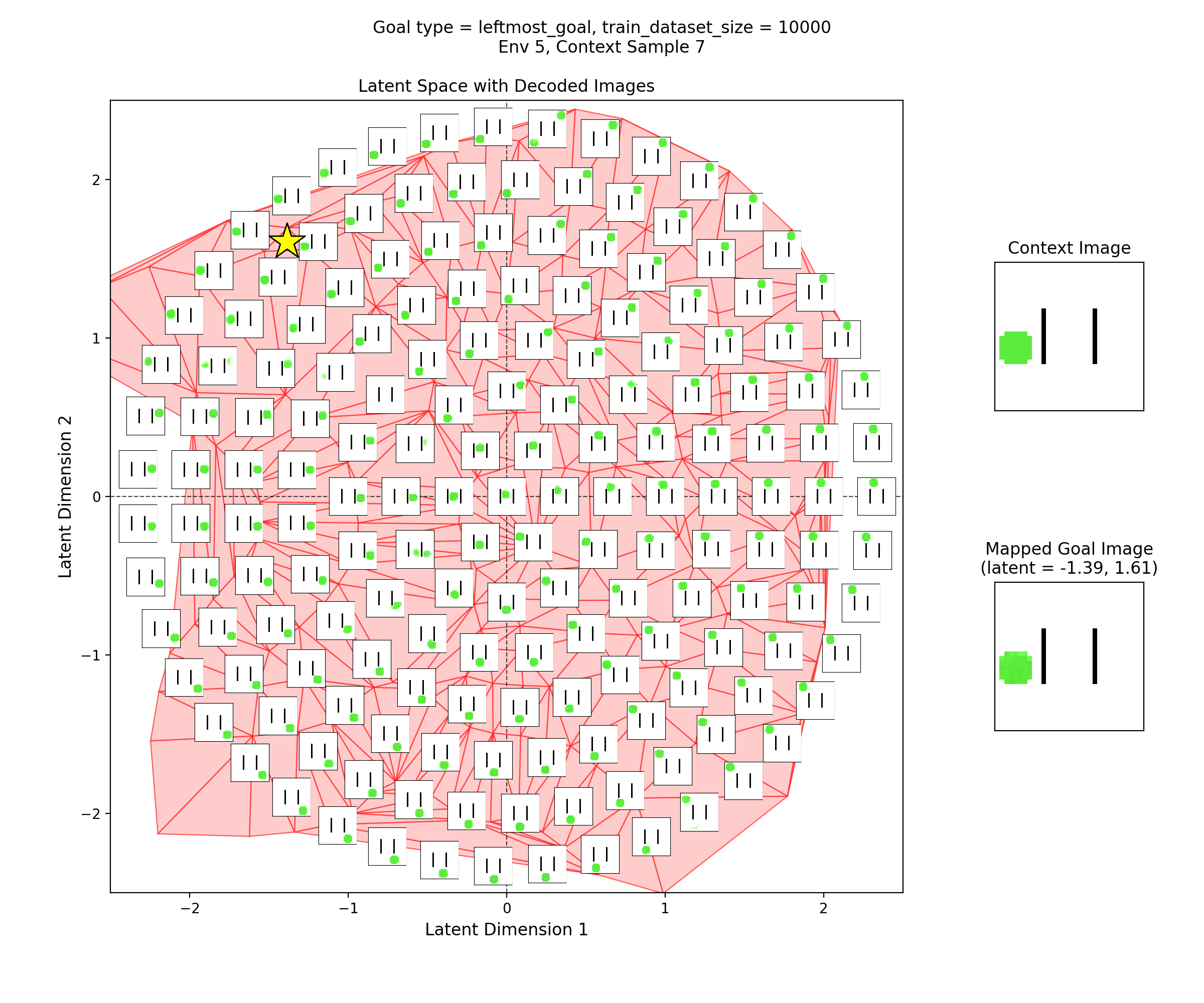
Then, I’ll show a few 2D latent space plots, basically the same deal as the ones above. However, in these ones, I’ve added a star to mark the point in the latent space that the context was mapped to, i.e., the latent goal. For all the goal types, I’m using the same RNG seeds, so we can see it move the same states to the different goals.

Upper left goal

Not super interesting, so just showing one context from each:

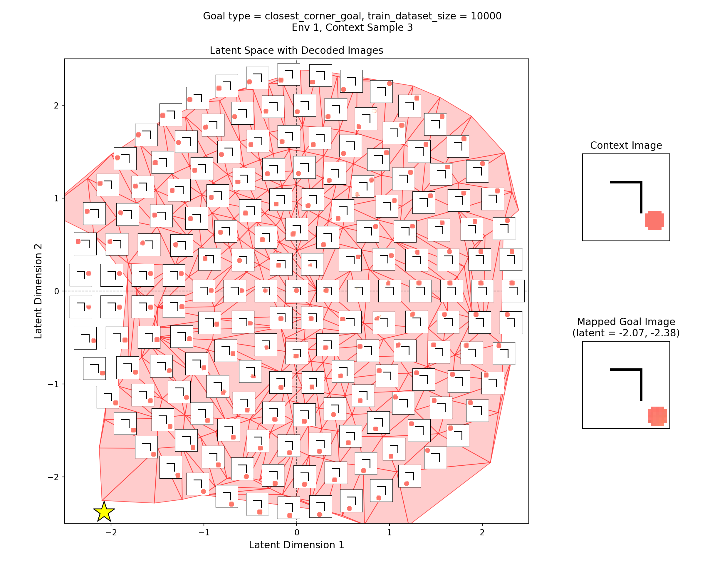
Closest corner goal

Leftmost goal

General observations

You can see that the latent space has some structure:

i.e., the origin in the latent space corresponds to the circle being at the center of the image, and you can distinguish some latent regions that correspond to the circle being in the corners.

You can also see that the triangulation (red shading in background) of the encoded real data points matches pretty well with the 2.5 standard deviation radius circle of latent points I’ve decoded for the inset images. That’s good, because it should mean that the vast majority of points we sample from the prior should get decoded to be real looking samples.

Lastly, you can see that the goal latent value is chosen about as well as it can be, from what I can see in any of the inset images in the latent space.

Scaling with dataset size

One more thing I wanted to test is how the performance scales with the size of the specific goal type dataset. This is important, since the assumption is that the CCVAE can be trained with a large amount of collected data from the environment in an “unsupervised” way, but the latent goal mapping model will need specifically chosen data.

For example, maybe you have hundreds of hours of footage of a video game being played, where the players weren’t playing with any particular goal type. This data is “cheap” and the CCVAE can be trained with it, but when we want to train the latent goal mapping model for a specific goal type, we’ll now have to provide examples of the goal being achieved. This is more akin to typical “supervised” training, where someone/etc will have to actually label some of that footage as achieving the goal. This is not cheap, and aside from that, we may just not have many examples of the goal type.

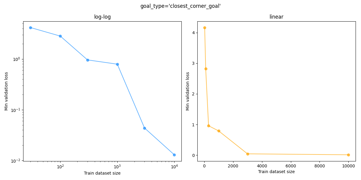
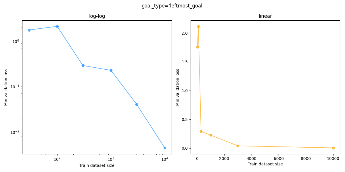
To test this, I took the same CCVAE, and trained the latent goal mapping model with (train) dataset sizes in ${30, 100, 300, 1000, 3000, 10000}$, for each goal type. We can then plot the min validation loss vs dataset size. Here that is for each goal type, where I’ve plotted both a log-log and a linear plot for each:

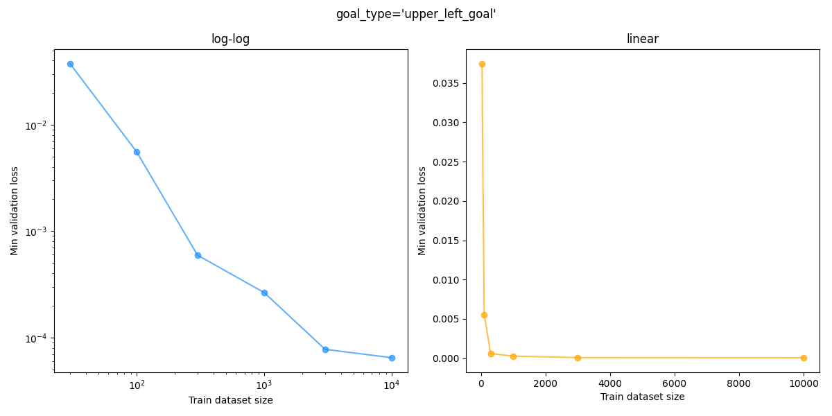
You can see that the “sanity check” static upper left goal loss gets down to the $\approx 10^{-2}$ range with even $30$ datapoints while the other goal types need much more data to get that low, which makes sense because it’s so simple.

However, a given validation loss value doesn’t tell us much in a vacuum; it’s the MSE in latent space between the mapped value and the true latent space value. To get a better sense, we can look at the goal reconstructions (like above) to get a sense for which MSE values are visually “good”.

For example, the size $30$ upper left goal looks like this:

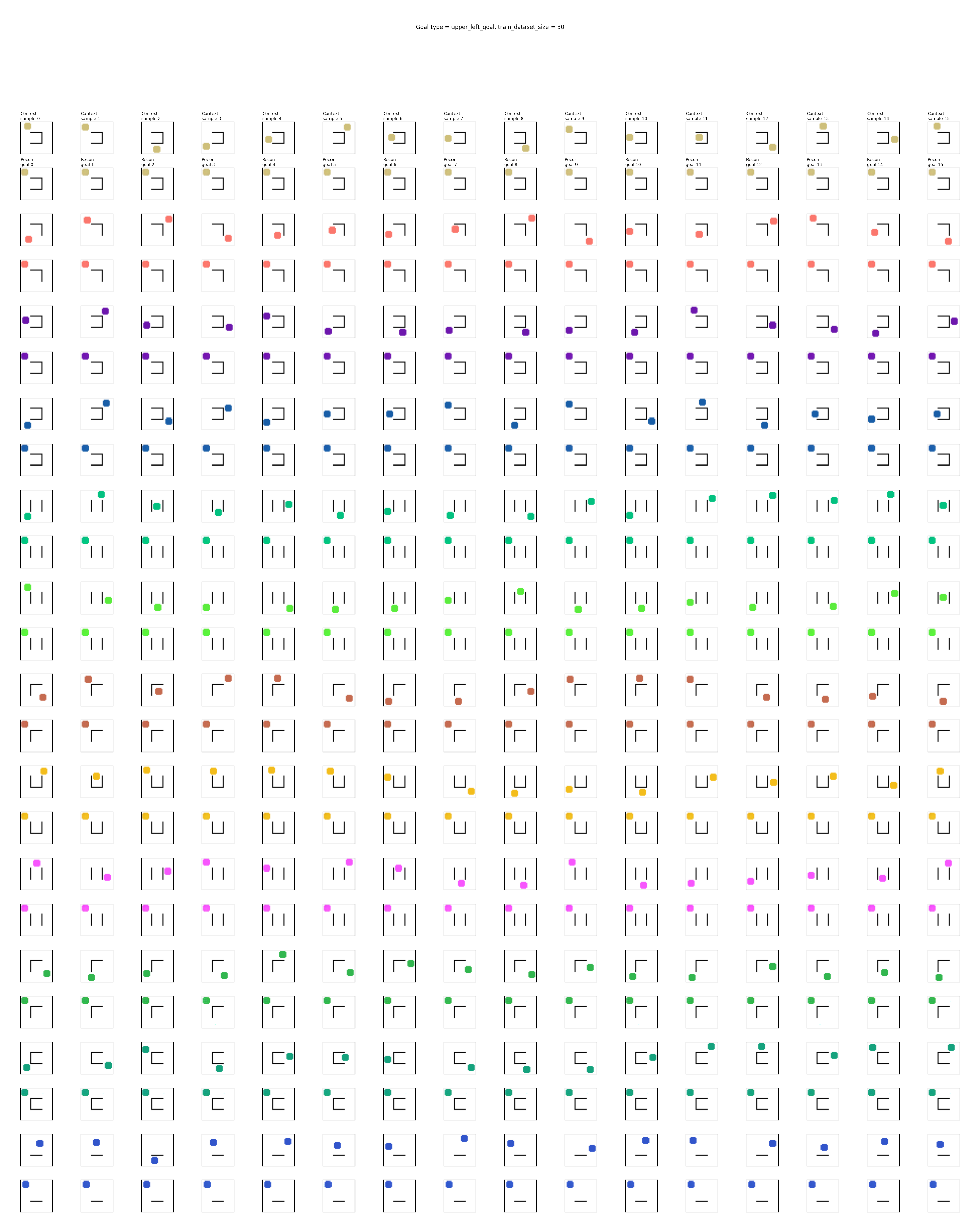
So, clearly that MSE is low enough in that case. But how low does it need to be for the others?

For the “closest corner” goal, it is useless at $100$, a little learned but pretty bad at $300$, mostly good but has a few errors at $1000$, and $3000$ looks very good:

For the leftmost goal, it’s about the same, though $300$ and $1000$ are a bit better. Here’s $3000$ for that:

I’m not sure how much of a win this is… for reference, the CCVAE itself was trained with a train dataset size of 100k, so if we need 1k goal examples, that’s 1% of 100k, which is relatively large in my opinion. I mean, in the wide scheme of dataset sizes, 1k is tiny, but this is also a tiny toy problem.

Discussion and thoughts

The structure of the latent space

Above I mentioned the structure of the latent space. However, there are some strangenesses. Here’s the image from that again, since I’ll refer to it:

Topology is a helluva drug

For example, looking at the image above, you can see that while the latent origin corresponds to the centered circle image, and there are distinct “corner circle” regions of the latent space, those corner circle positions/directions aren’t maximally separated from each other or orthogonal or anything, like you might intuitively expect.

In fact, you can see that the bottom left corner and upper right corner are both mapped to nearly the same region where the star marker is in the image above! So they’re not just not separated, they’re actually right next to each other. What’s going on?

I think the possible answer is pretty interesting. To keep this short (lolz) I’ll do a separate post on it some day, and for now just say that I think it’s fundamentally a topology problem: the latent space is like $\mathbb R^2$, but the data image space is like $\mathbb R^2$ with a few “holes” in it, because of the walls. This makes the VAE’s job really hard, and the best it can do is map some very different images (i.e., the bottom left and upper right corner circle images) to bordering regions in the latent space.

To cover the latent space well, it should want to make the “separating” region in the latent space between (the latent space regions of) these very different images as slim as possible, which it seems like it mostly does. However, if you look at the inset image directly to the right of the star above, you can see a decoded image that has two circles! This is because while it looks like that’s an image covered by the Delaunay triangulation of the real data, it’s actually in that region between the latent values of two of them; on either side, the decoder knows how to decode them into real samples (as you can see it does well), but for that slim region, it doesn’t correspond to any real data, and decodes it as a mix of the two regions, i.e., an image with… two circles!

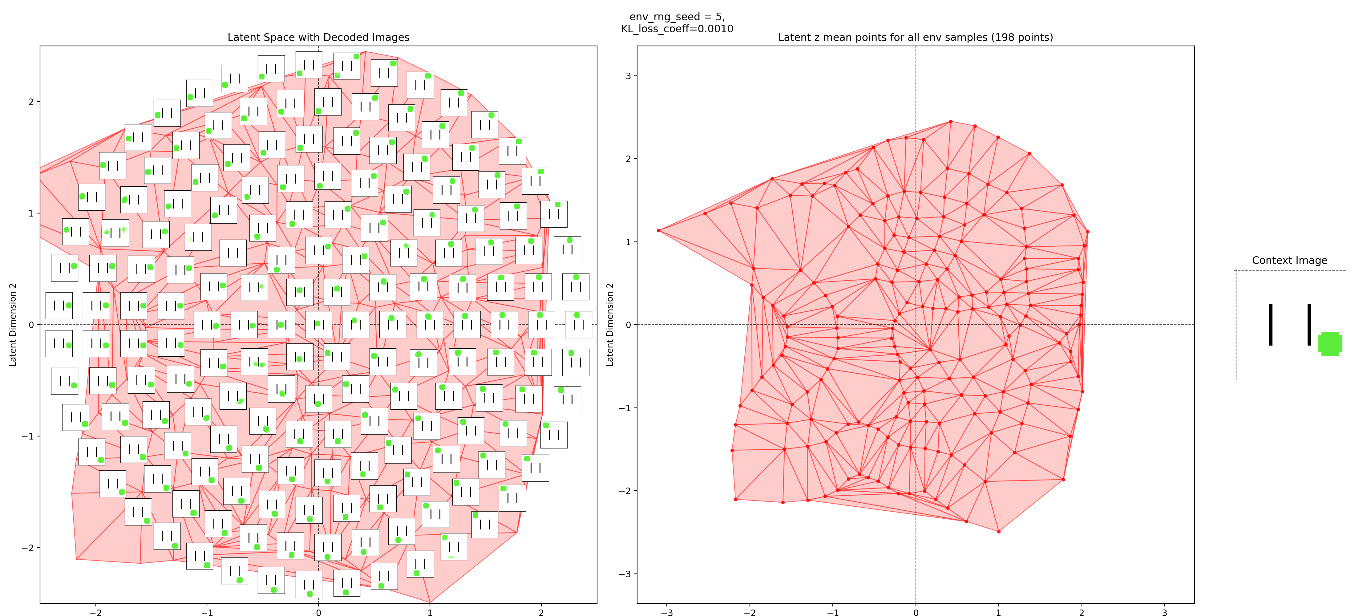
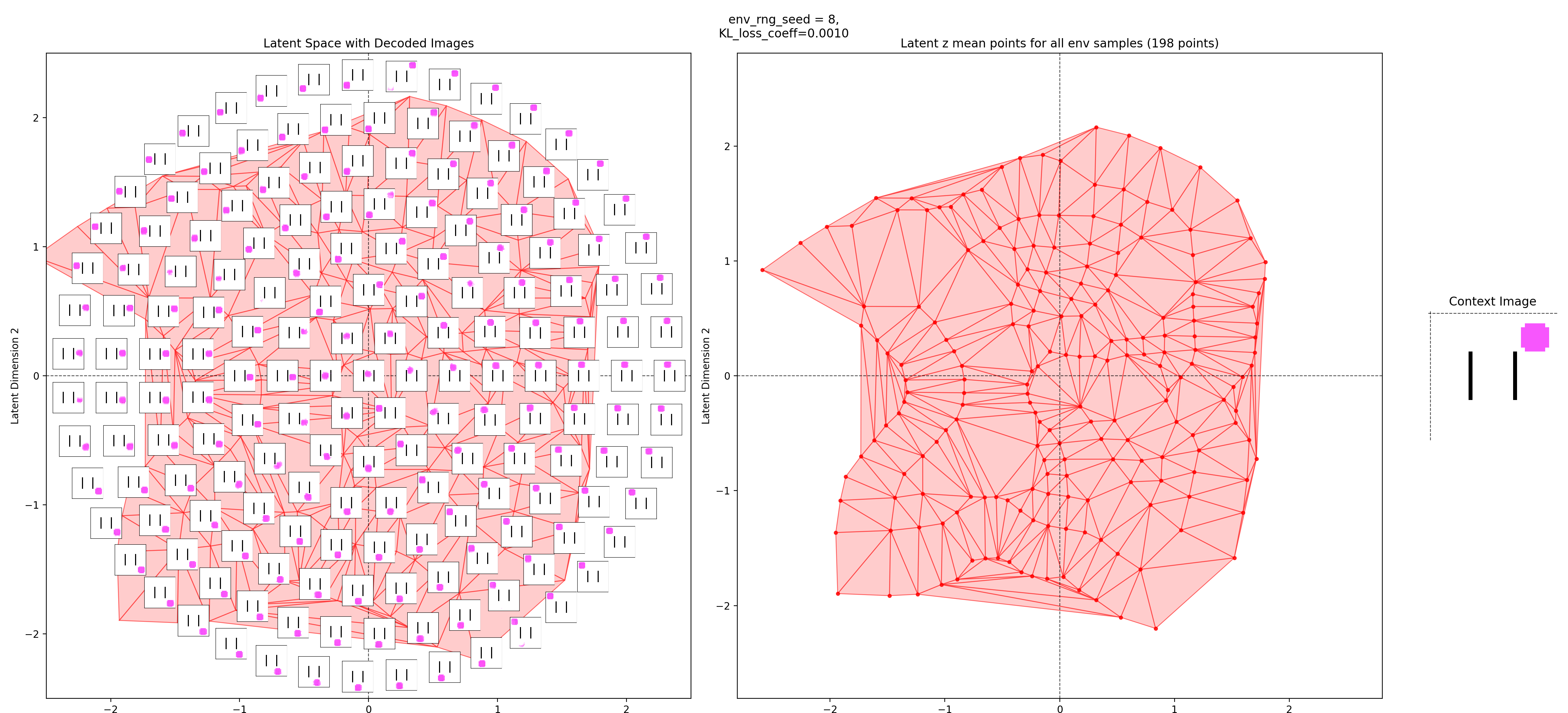
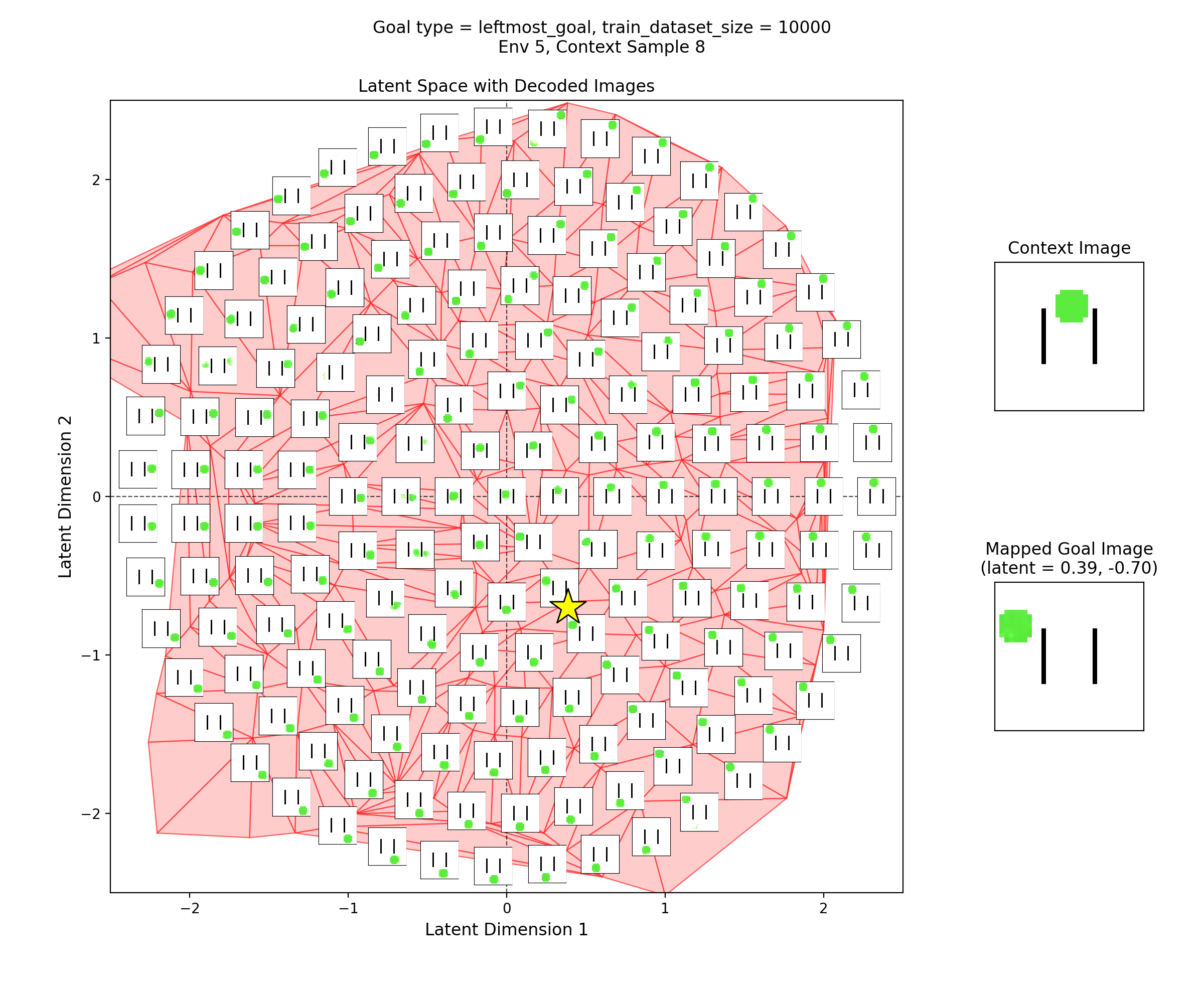
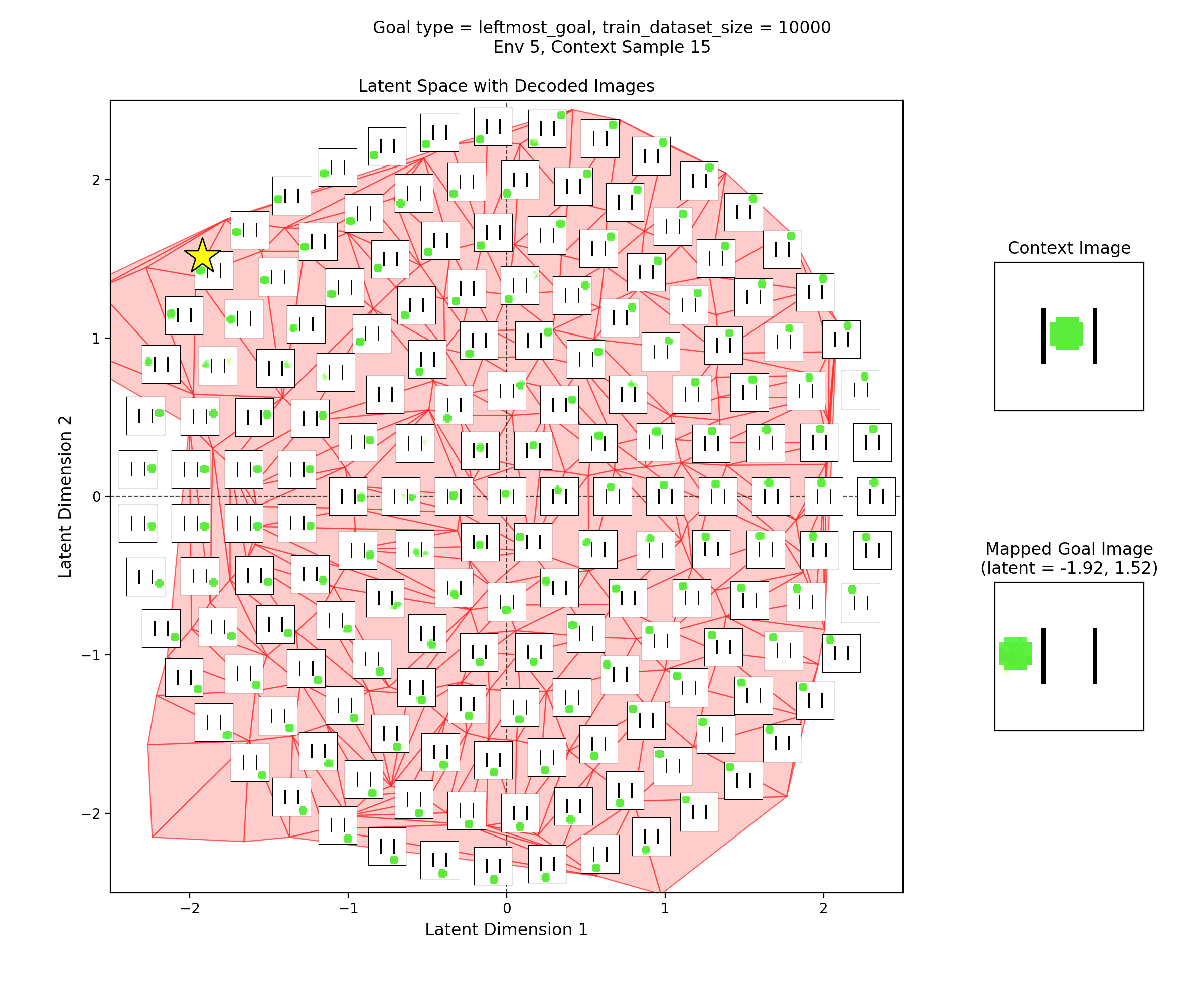
The context position doesn’t seem to change the latent space?

I’m not sure this is wrong, but it did strike me as weird and makes me wonder if I’m doing something wrong. If you look at two of the latent space images above, for the same env but different contexts, you can see that the different latent space locations get decoded to the same images. E.g., for the green circle with two vertical walls env above, $z = (1.5, -2)$ decodes to the circle in the upper left, regardless of where the context circle was.

Obviously, when the context is a different env, the same $z$ will produce a goal image for that env. But this means it’s basically just encoding the circle color and wall positions in the latent context and throwing away the context circle position. In fact, even for different envs, you can see above that the same $z$ value still mostly corresponds to having the circle at the same position in that env. Since some envs have valid circle positions that are invalid for other envs, they move around a bit to accommodate this, but they’re mostly the same.

Intuitively, I expected what $z$ means to be very dependent on the context circle position too. For example, I was expecting $z$ to kind of act as a “modification” to the latent context, such that $z = 0$ would result in the same image as the context, and nonzero $z$ values to move the circle around with respect to that.

However, I think this makes sense, given what we trained the CCVAE to do. The training pairs are just two samples from the same env, where one is the context and one is the goal. Therefore, we’re basically saying saying that any valid state can be a goal from any other state in that env, and it really doesn’t need the context position at all. If I had trained it on a more restrictive set of state/goal pairs like the ones I trained the latent mapping models on, where the distribution of goals does depend on the context position, then I’d expect them to have different latent space meanings. Maybe something to confirm in the future.

VAEs kind of suck?

This was one of those things where I did like 90% of the project pretty quickly, and then proceeded to tear my hair out for ages on a pretty small aspect. It’s good to show how the sausage is made sometimes.

When I was implementing the toy env, I just looked at their examples image (above) and said “yeah yeah, some black lines and a colored circle, gotcha”. So I implemented that, using a few simple rules for placing the walls, how big they can be, placing the circle, etc. That implementation gave envs like this, for example:

And… I dunno, those look good, right?

However, when I trained with these… well, it kind of worked… kind of. It could typically reconstruct data samples fairly well:

but, when I went to sample the latent space and reconstruct those, I’d get stuff like this:

You can see that for all of them, the walls are in the correct place and the circle is the correct color. And, many of them are basically plausible states. However… there are also some that are clearly messed up, where it has just placed the circle on top of a wall.

After messing around a bit, I kind of suspect that it basically learned to reconstruct the context, but also place the circle anywhere, with no concern for walls. If this were true, most of the time the circle wouldn’t intersect any wall, which would be a valid sample. But it’d also mean it hasn’t really captured the env in as meaningful a way.

Looking at the latent space diagrams from above, they were also producing weird stuff like this:

in which no data was being placed at some of the highest density regions of the prior, and there are weird separate “chunks” of the embedded data. This is why the latent samples for this are bad, by the way – as I talked about above, all those regions in between where the latent values of the true data points don’t correspond to actual data (see their reconstructions in the left plot), so the decoder has trouble with them.

I spent longer than I’d like to admit going nuts with this, trying all sorts of architecture changes and other stuff, mostly to no avail. I finally went back to the paper to see if there were any details I missed; I was mostly curious if they were using some massive dataset compared to what I was using or something. They used about the same size dataset (~100k samples), but what I did notice was:

The arrangement of the walls is randomly chosen from a set of 15 possible configurations in each rollout, and the color of the circle indicating the position of the point robot is generated from a random RGB value. Thus at test time, the agent sees new colors it has never trained on.

(They don’t say it explicitly, but if you look at the example image above from the paper, it was pretty easy to infer that the “15 possible configurations” are actually just 4 walls that form a box in the center, and they choose between 0 and 3 of them each episode. If you sum (4 choose 0) + (4 choose 1) + … + (4 choose 3), you get… 15.)

The point is that 15 configurations are way, WAAAAY fewer than the number mine was producing! This made all the difference. It was pretty much night and day, where it immediately produced the good images I presented above. I also suspect this is exacerbated by the topological problem I mentioned above, moreso for my toy env version, but that’s for another day.

However, this is still a bit disappointing to me: my original toy env implementation is still pretty simple as far as environments go, and it seems like the type of thing the CCVAE should be able to capture well enough. My best guess is just that the increased number of envs would require a ton more data to learn the pattern well, and VAEs are kind of a blunt instrument.

An unsatisfactory part of the whole “vastly simplifying the toy env made it work” is that I worry we basically just memorized the whole dataset. This toy env is very structured, so ideally we should be able to see a subset of all the possible envs and contexts, and generalize to unseen ones. However, after using the simpler one I realized that it’s now so limited that we may basically be showing it the vast majority of possible samples. There are 15 different wall configurations. For each, there are $\approx 200$ valid circle positions IIRC. That gives 3k wall/position samples. The circle color is a mostly unrestricted continuous RGB value. But, the train dataset size was 100k, so if we discretized the color space to 30 different colors, we’d have roughly as many training data samples as there are. There are obviously more than 30 colors and I’m guessing the dataset has many duplicates, but even being in the ballpark of it is a distinctly different regime.

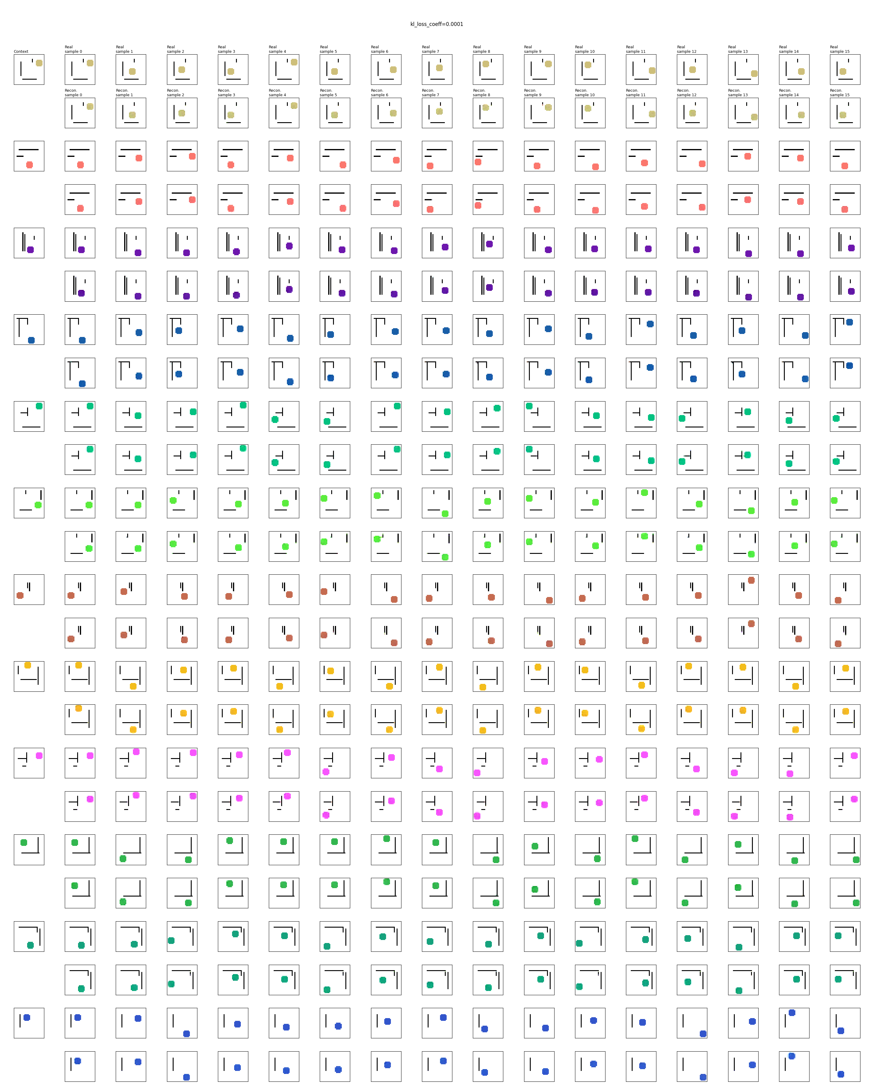
KL annealing

One last thing on this front: in my desperate thrashing while trying to solve the problem, one thing I tried was annealing the coefficient of the KL div loss term. I’d been aware of this trick for a while, but never actually tried it before. I’m not sure if this is kosher or what, but I basically modified my early stopping callback so that when it does early stopping based on the validation loss no longer dropping, that’s when it increases the KL coefficient to the next stage (and restarts the early stopping from there).

And let me say, it definitely helped! It really seems like training without annealing (i.e, just starting with a given KL coeff) can lead to some really lousy results if the coefficient is high. On the flip side, starting with effectively no pressure to match the prior seems to let it first concentrate on learning the encoder and decoder well enough to reconstruct, and then it’s a lot easier to add the incentive to match the prior once those are learned.

We’re not actually doing RL here, should we be?

The CC-RIG paper is all about doing this for the purpose of generating meaningful goals for helping the learning process. Above I mentioned that despite this, although I’m actually not doing RL here, I think it should be fine because my purpose (goal?) is generating a specific type of goals, and I’m assuming that the policy can go to any real goal already. Therefore, it’s not super relevant for what I want.

But is this true? I can think of at least two reasons it might not be (not that that means I’ll be doing it today though :P).

One is that the way I was judging how well the goals were produced was by looking at a few metrics related to how well it hits the “target” (whether that was the latent goal, or a reconstruction, etc). That seems reasonable, in the sense that if it does that perfectly, it’s probably doing a good job. But it could be leaving a lot on the table. The policy is a complicated beast, and we don’t know how it’ll necessarily respond to different latent goals. For example, it’s possible it’s actually much more “forgiving” for some variation in parts of the latent goal, and then we might be over/underoptimizing the wrong parts of our goal proposal models.

The second is kind of just a more general version of the first. We don’t actually care about proposing latent goals for the sake of doing that. We want them to use with the policy. The more general point is that we can’t really say if we’re succeeding or not unless we know it’s working well for the actual use case. Even if it seems like it “should” work great, we really need to test it with the actual purpose for it to know. It can go both ways, where there’s something about the approach we didn’t expect that makes it terrible, even if the “primary” metric we were looking at says it should be great, or it could be better than expected (like in the 1st point).

Do we really have to do all this? Couldn’t we just learn a direct mapping from state to goal images?

This might all seem like a lot of work for something relatively simple, and you might reasonably ask “can’t you just directly train a model that maps the state to the goal state?”

This is a good question. Keep in mind that the raw states here are images in general, so that would mean being able to predict one image from another, and we don’t have a ton of ones to train on.

I didn’t test this here, but partly because I think it might actually work in this case, but it wouldn’t show much. These images are shape $(32, 32, 3)$ or so, so I think it’s plausible it could learn to do it, but maybe not for larger images.

Can GPT just do it?

That said… diffusion and Visual Autoregressive models and all the fancy new toys are really good at things like inpainting, modifying images, etc, which is kind of what this is doing, in this simple case at least. Out of curiosity, I tried to see if GPT-4o could one-shot it:

Maybe asking for a 10x10 grid was asking for too much?

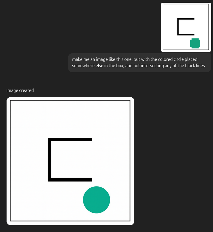
Huh! Maybe I still have a job, for a little while anyway.

Aside from this though, there are a few reasons this doesn’t actually solve the problem: 1) not all envs would have the goal state image be so similar to the current state image. For example, in a video game env, the goal could be traveling to a different region and using an inventory item. 2) We don’t necessarily care about producing images! Like I mentioned, usually these methods have the RL models working in the latent space anyway. 3) Most importantly: the whole point is to learn the structure of the environment. We don’t just want to produce other states, we want to produce sensible states given the context.

Next time

Next time, I’ll try a slightly less simple method for producing the latent goal states. As a teaser, this will probably be a method based on a combination of ideas from Contrastive Learning as Goal-Conditioned Reinforcement Learning and papers like Generalization with Lossy Affordances - Leveraging Broad Offline Data for Learning Visuomotor Tasks (i.e., “FLAP”). I might also use something besides a VAE to do the embedding, since I’m kind of sick of VAEs at this point.