Generalized graph drawing - simple is smart!
Previously, I implemented the paper “The Laplacian in RL: Learning Representations with Efficient Approximations”. Today I’ll show some results of implementing a follow up paper from different authors, “Towards Better Laplacian Representation in Reinforcement Learning with Generalized Graph Drawing” (2021).
The method in the newer paper is a shockingly simple extension to the previous one (“Laplacian representations hate this one weird trick!”), so this should hopefully be shorter. But it’s also piggybacking off the previous paper a lot, so check out that post first.
Brief background, main idea, motivation
As I stumbled upon back when I wrote about the graph drawing objective / quadratic form of the Laplacian, if your objective for finding eigenfunctions of the Laplacian only contains the energy minimization term $E(F) = F^\intercal L F$ (where $F$ is a matrix of $d$ stacked candidate eigenfunctions) and an orthogonality constraint penalty $\beta \cdot \Vert F^\intercal F \Vert^2$, then you’ll find solutions that do minimize both $E(F)$ and the constraint penalty!
However… the whole energy is actually the sum of the energies of each of the eigenfunctions, $E(F) = \sum_i^d E(f_i)$. The true eigenfunctions $f_i$ will have the property that each $E(f_i)$ is as small as possible, while being orthogonal to all the previous/other ones. These not-true-eigenfunction solutions have the same sum $E(F)$ as for the true eigenfunctions, but different individual $E(f_i)$. Borrowing a plot from that post, that looks like this:
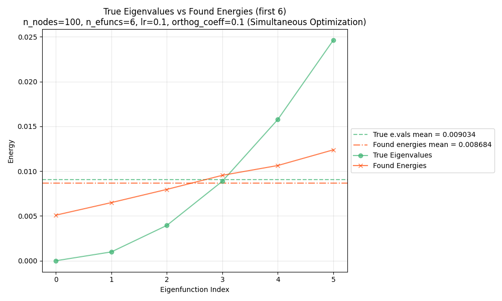
You can see that the learned eigenfunctions have effectively the same mean $E(f_i)$ for the first 6 eigenfunctions as the true eigenfunctions, but that energy is “distributed” differently across them.
And in fact, in the post for the predecessor paper of the one today, we also saw this for the eigenfunctions it found! Below:

In the quadratic form post, I mentioned two ways this can be mitigated. One way is an after-the-fact method that worked well, but I’m pretty sure can’t easily be applied to real problems with large/continuous state spaces. The other way is something that should theoretically work for real problems, but I was having trouble getting it to work, even for that simple problem.
This is the problem today’s paper is trying to solve: on its own, the graph drawing objective (GDO) doesn’t find the true eigenfunctions, and we want those tasty true eigenfunctions!
Like I said, their method is so simple that I feel a bit dumb for not thinking of it myself. And to be clear, that’s not a knock on them at all! In fact, it’s all the more clever. Here’s what they did: instead of the energy term $E(F) = \sum_i^d E(f_i)$ in the objective, they added a coefficient to each energy term: $E(F) = \sum_i^d c_i E(f_i)$, where ${c_i}_i = {d, d-1, \dots, 2, 1}$.
That’s it. That’s literally all.
Why does this work? Intuitively, the problem was that although the original GDO minimizes the sum $E(f)$, it’s agnostic to how the energy is distributed among the individual terms. Adding these coefficients changes that fact: now if you consider a solution where it has successfully minimized the sum $E(f)$ but not the individual components, it does care about the way the energy is distributed, since $E(f_1)$ has a coefficient of $d$ and $E(f_2)$ has a smaller coefficient of $d -1$. Therefore, the optimization problem should find $f_i$ such that $E(f_1)$ is as small as possible.
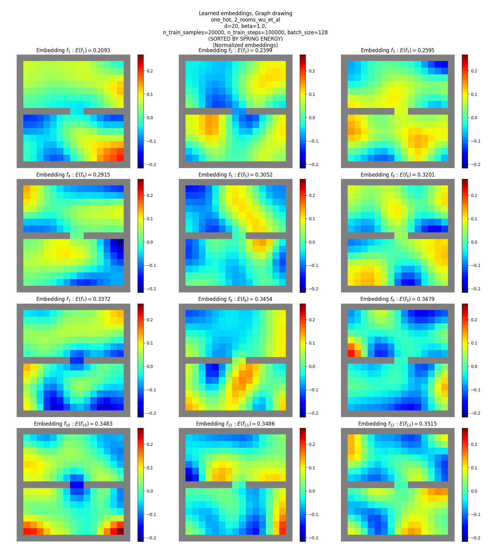
Why do we even care about this, though? Well, partly, it’s just cooler to actually find the true eigenfunctions, if possible. But a more practical reason is that a set of the true eigenfunctions capture some structure that a rotation of that set might not. If you look the learned eigenfunctions I found in the predecessor paper post last time:
to the true eigenfunctions:
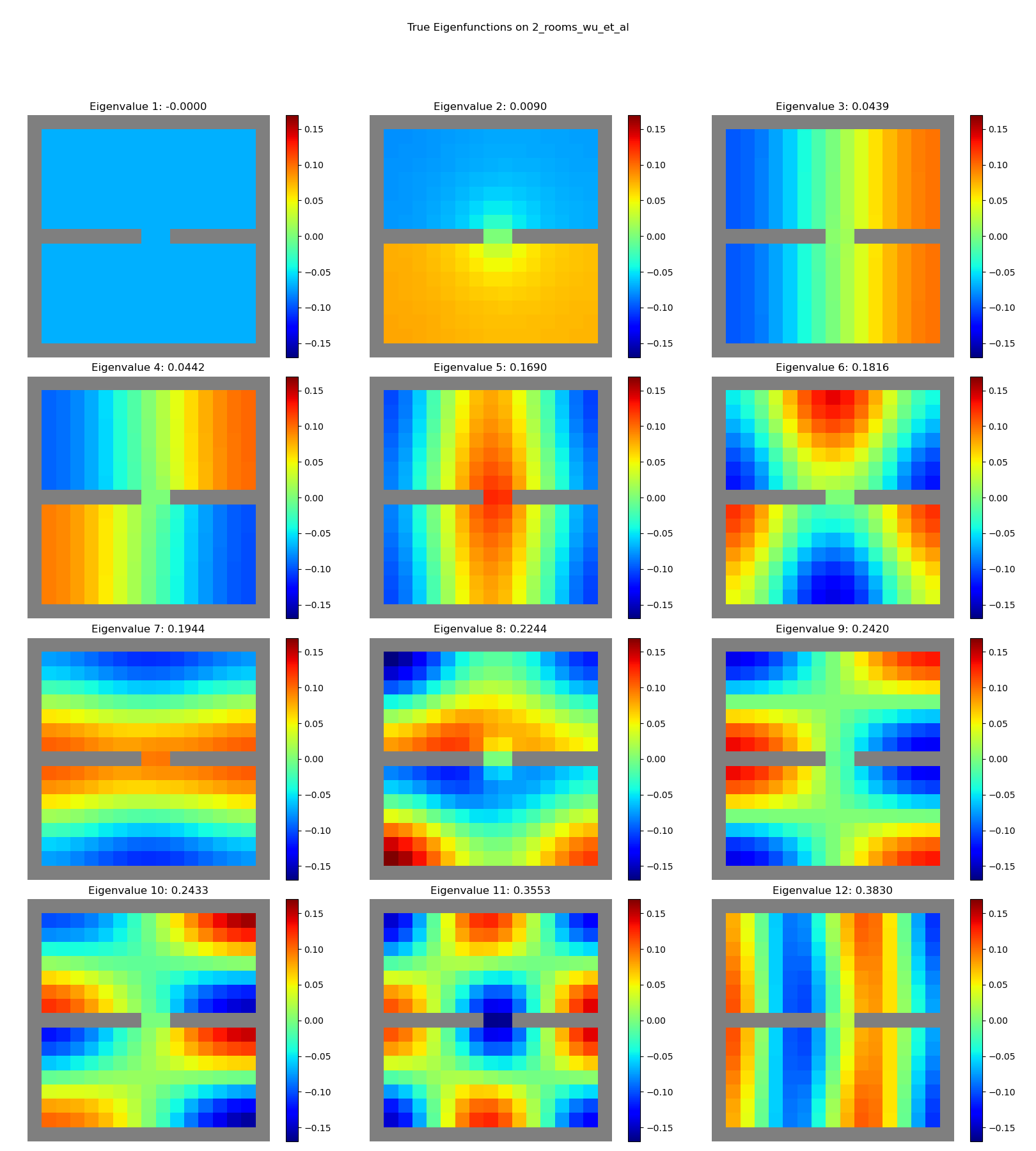
You can see that the true ones have obvious meaningful shape to them – for example, if you followed the gradient of one of them, or traversed an equipotential of it, it’d plausibly lead you to more interesting states. Meanwhile, the learned ones are mostly random blobs.
Experiments
They do most of the same stuff as the predecessor paper (which I’m calling “baseline” or “Wu et al” here, and I’m calling their method “GGDO”). However, they test with slightly different environments:
- they use two different discrete mazes,
GridRoomandGridMaze(see below) - they use two different continuous control mazes,
PointRoomandPointMaze(also below)
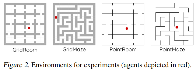
Note that these are more complex than the ones in the predecessor paper:
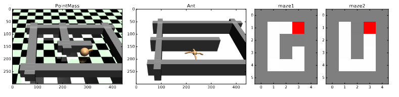
For state representations (i.e., inputs to the models), they learn the discrete mazes with coordinate $(x, y)$ representations and image/pixel representations. For the continuous mazes, they only use coordinate representations.
There are some other details (which they’re a lot clearer on than the original paper), and some minor differences: they always use multi-step discounted transitions with $\lambda = 0.9$, and their batch sizes are a lot larger ($1024$ for discrete, $8192$ for continuous). They find the first $d = 10$ eigenfunctions in all cases.
Their main takeaway image for selling you on the method’s success is comparing the $d$ learned eigenfunctions to those found for the Baseline method, as well as the ground truth. Here’s their image:
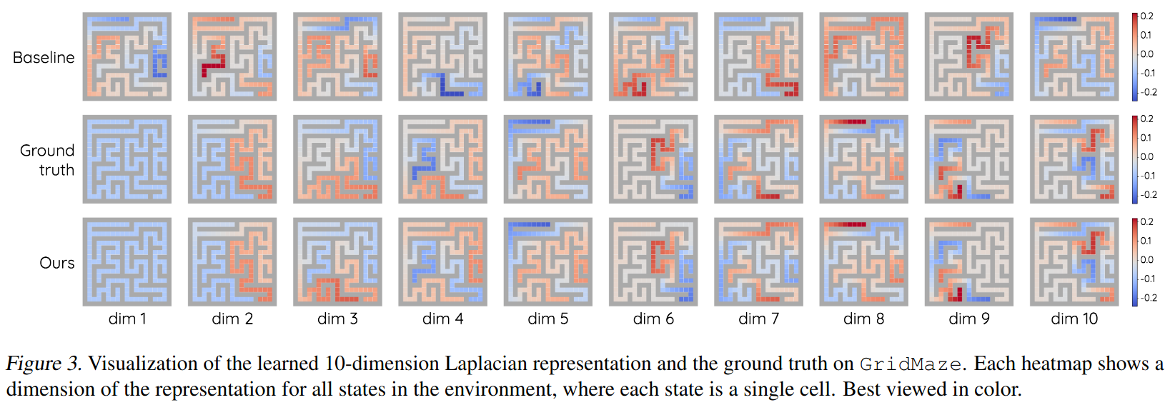
Row 3 looks like Row 2, Row 1 looks… different. Here’s what I found:
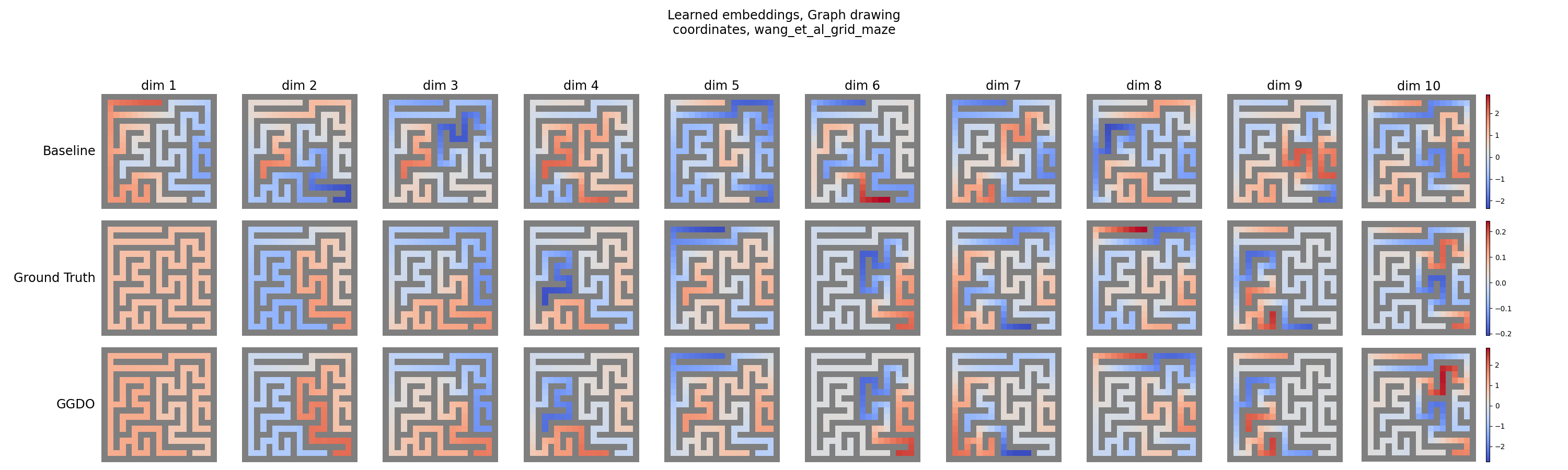
Heyoooo, pretty close! You can see that some of the colors are flipped from theirs, because they’re the same up to sign. I just made it so the learned ones match the signs of the ground truth. You can see that mine both match the ground truth, but also match theirs quite well.
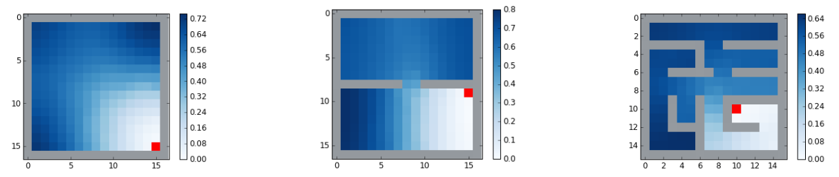
GridMaze is discrete though. Here’s their image for PointRoom, which is continuous:
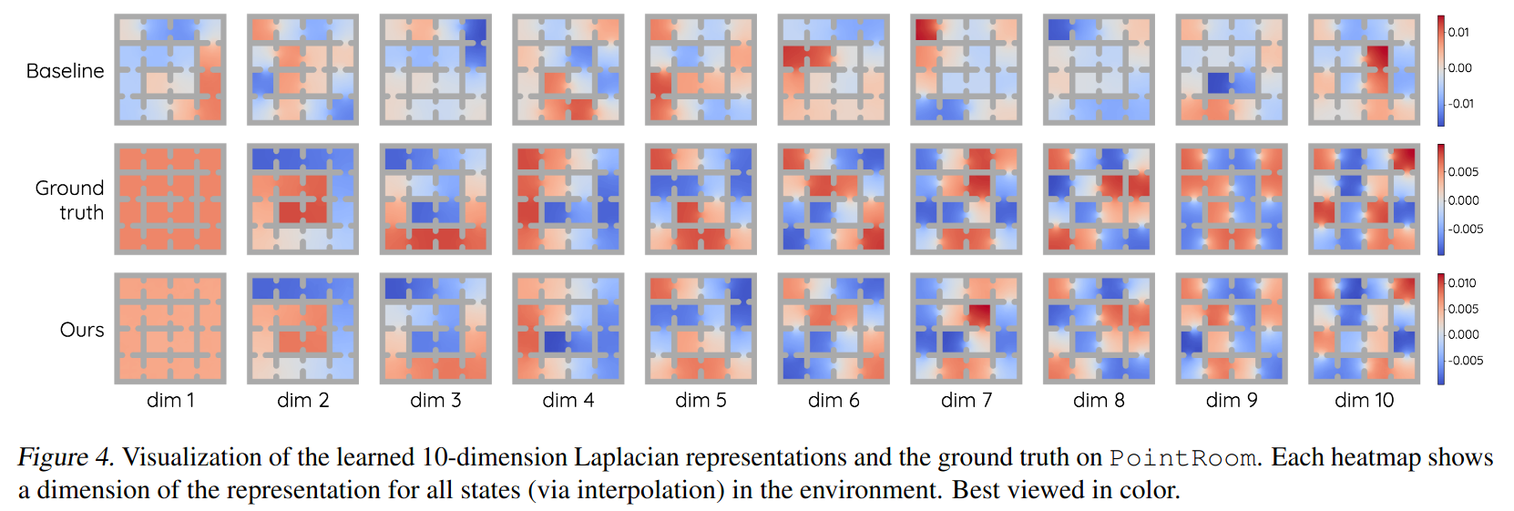
And here’s mine:
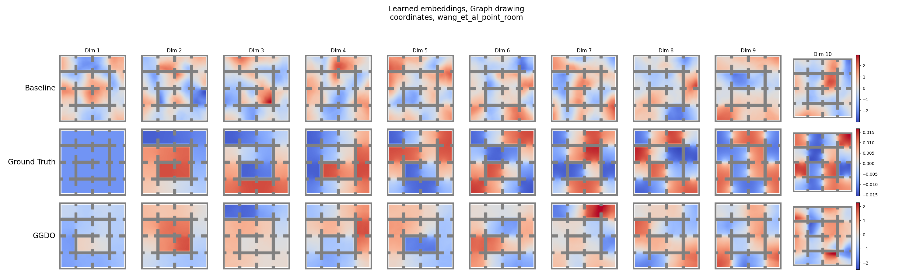
Hmmm, not quite as good, but still much better than the baseline, and mostly matches the GT. More on that below.
However, these are kind of qualitative. Next they define some metrics which let them actually say “look, number $X$ is bigger than number $Y$, our method is better”. First, they define the “SimGT” metric:
\[\textrm{SimGT}(f) = \frac{1}{d} \sum_{i=1}^d \bigg\vert \sum_s f_i(s) e_i[s] \bigg\vert\]$f$ is a candidate solution of $d$ learned functions $f_i$, and $e_i$ is the $i$th ground truth eigenfunction. Basically, $\textrm{SimGT}(f)$ is in $[0, 1]$ and tells you how well each of the $f_i$ are aligned with the corresponding ground truth (GT) functions.
They also define the “SimRUN” metric:
\[\textrm{SimRUN}(l, m) = \frac{1}{d} \sum_{i=1}^d \bigg\vert \sum_s f^l_i(s) f^m_i(s) \bigg\vert\]This is the same idea, but it’s for measuring the alignment between two different training runs, $l, m$, which tells you how repeatable it is.
So with those defined, they (and I) train each of the envs above, with both methods, for both state representations (for the discrete envs), for three runs apiece.
That gives them this table, where they compare the SimGT for the two methods:
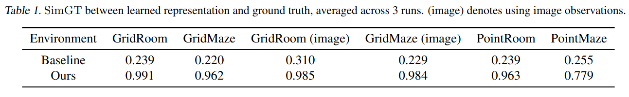
My results give:
\[\begin{array}{c | c c c c c} \hline \textbf{Environment} & \textbf{GridRoom} & \textbf{GridMaze} & \textbf{GridRoom (image)} & \textbf{GridMaze (image)} & \textbf{PointRoom} \\ \hline \textbf{Baseline} & 0.250 & 0.281 & 0.258 & 0.200 & 0.178 \\ \textbf{GGDO} & 0.989 & 0.982 & 0.918 & 0.809 & 0.556 \\ \hline \end{array}\]My GridRoom and GridMaze results are pretty close to theirs, though the image ones are a bit worse. My PointRoom results are a lot worse. I didn’t end up running PointMaze.
They also look at the SimRUN metric for theirs and baseline. To do that, they basically make these little matrices showing the SimRUN between the three runs for each run configuration:
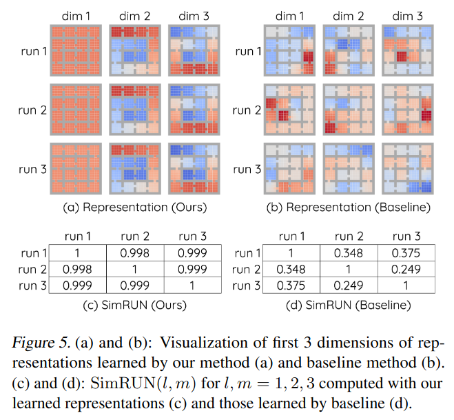
You can see that both methods have $1$ on the diagonal, since it’s the SimRUN of the the same run with itself, but theirs has way better off-diagonals, saying that the three runs independently found very similar solutions. Here’s what my results give for GridRoom:
My results, baseline:
\[\begin{array}{c | c | c | c | } \textbf{ } & \textbf{run 1} & \textbf{run 2} & \textbf{run 3} \\ \hline \textbf{run 1} & 1.000 & 0.195 & 0.256 \\ \hline \textbf{run 2} & 0.195 & 1.000 & 0.324 \\ \hline \textbf{run 3} & 0.256 & 0.324 & 1.000 \\ \hline \end{array}\]Ballpark similar enough.
My results, GGDO:
\[\begin{array}{c | c | c | c | } \textbf{ } & \textbf{run 1} & \textbf{run 2} & \textbf{run 3} \\ \hline \textbf{run 1} & 1.000 & 0.980 & 0.982 \\ \hline \textbf{run 2} & 0.980 & 1.000 & 0.976 \\ \hline \textbf{run 3} & 0.982 & 0.976 & 1.000 \\ \hline \end{array}\]Possibly slightly worse, but close enough for today!
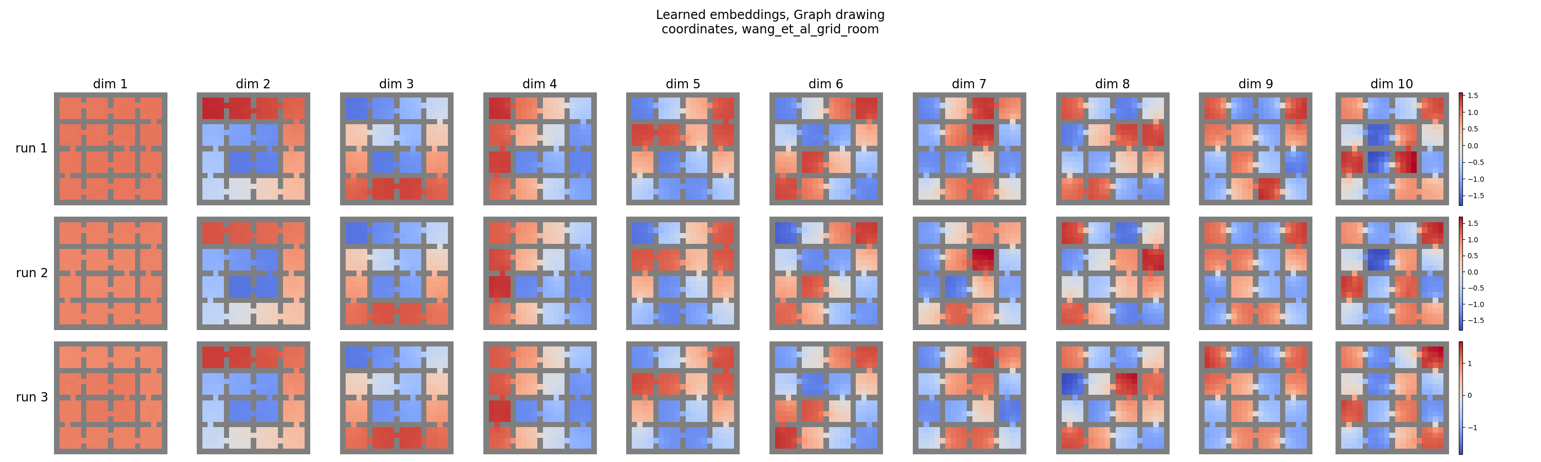
And we can see this by inspecting the learned embeddings across the three runs for each of the methods, as they show for $d \leq 3$ in Figure 5 above, or for all $d$ in the appendix:
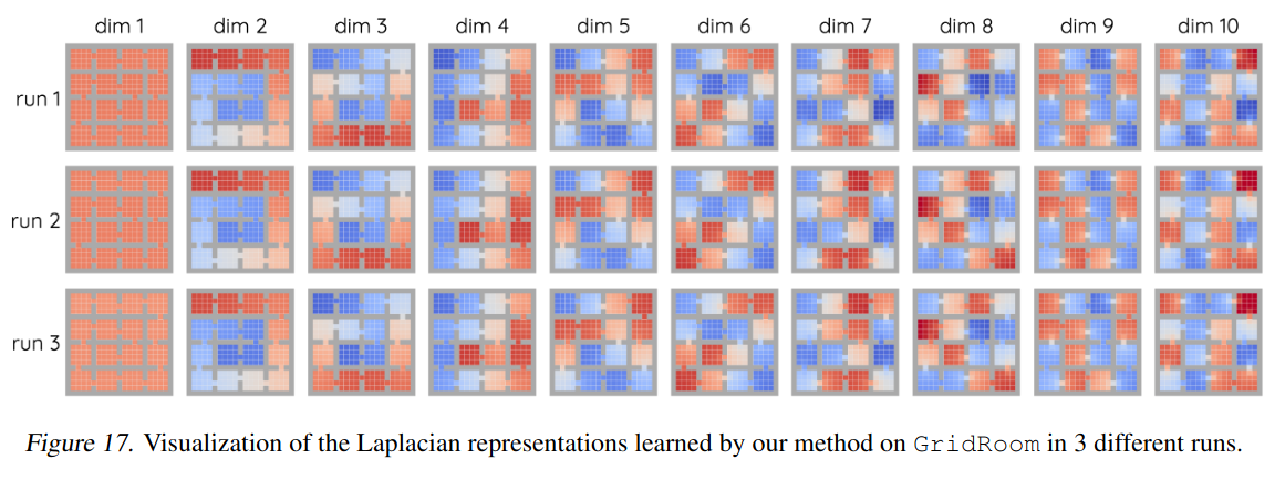
And here are mine:
GGDO:
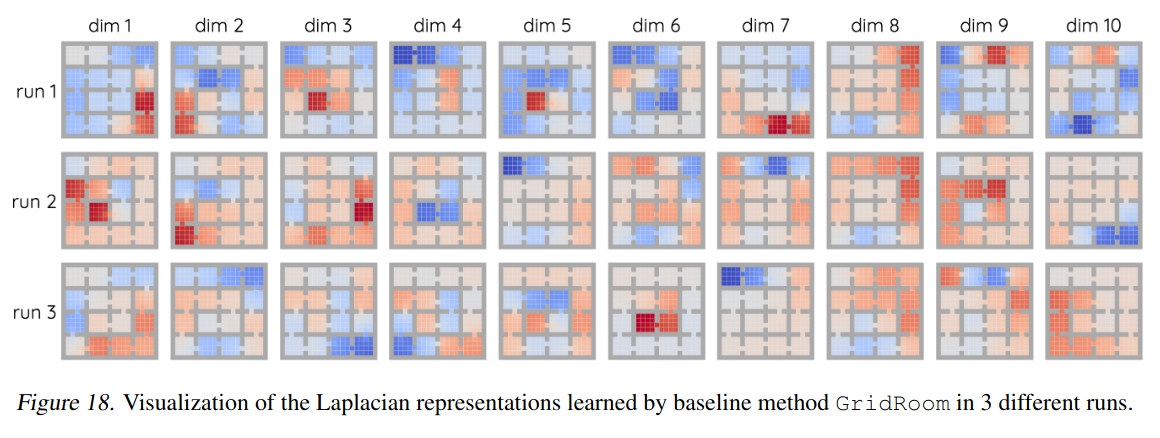
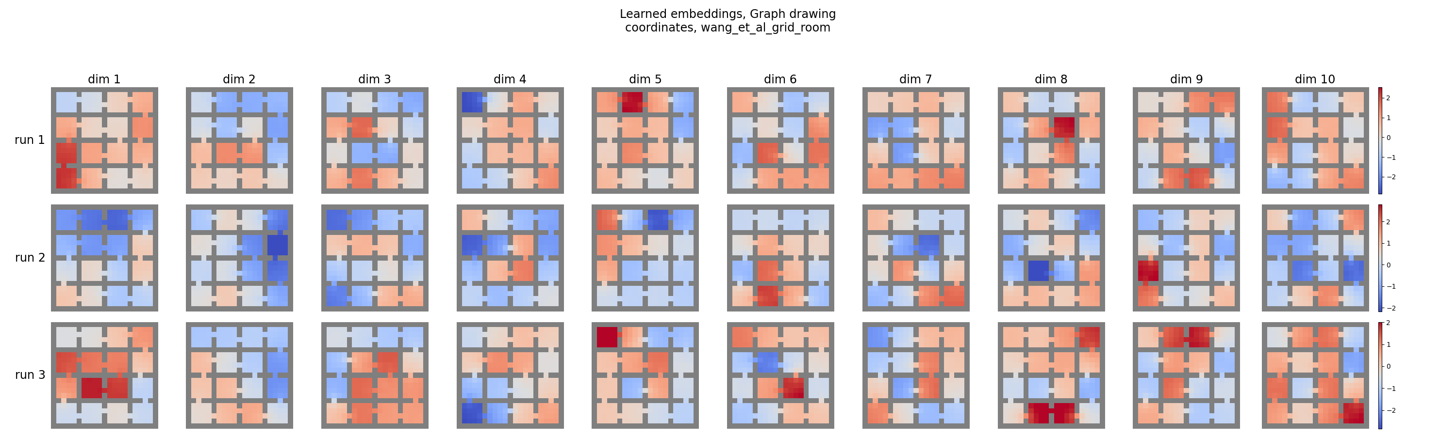
Baseline:
Yeeeehaw! You can see that the first ~6 look really similar for GGDO, and then there are a few slight differences for the higher order eigenfunctions. But overall, they look really good.
This should hopefully all make sense: in their GGDO method, there’s one way to get the lowest energy, so independent training runs tend to find very similar solutions. In contrast, in the baseline method, orthogonal rotations have the same energy, so there’s no reason the independent runs would converge to the same solution, as we see.
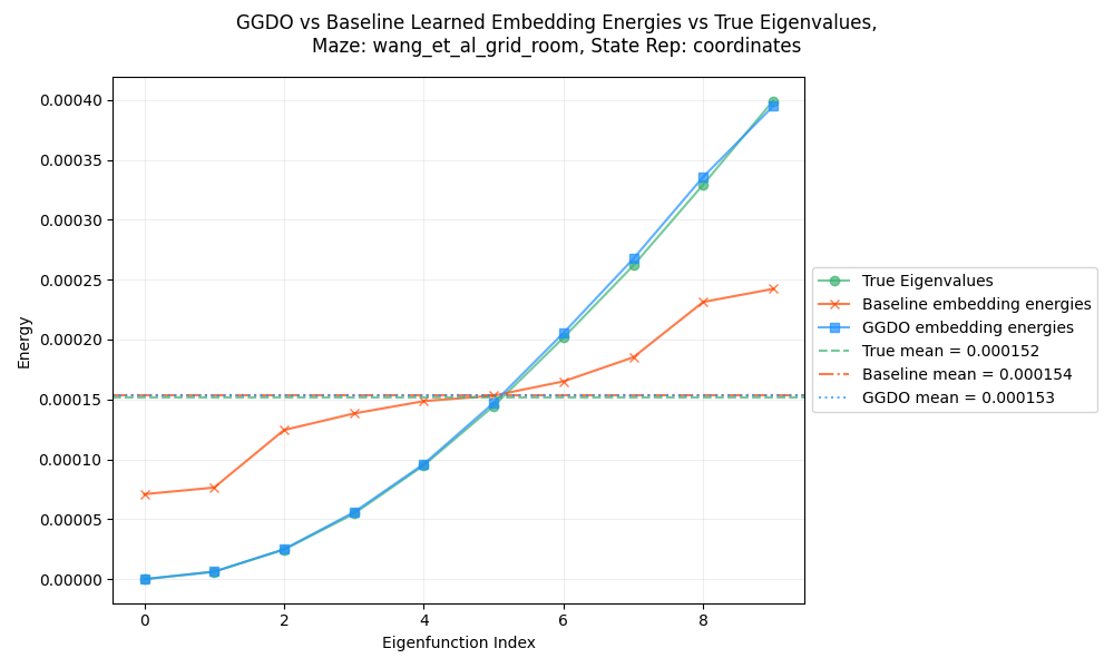
One last thing! Let’s look at the plots that we motivated things with before, of the individual functions energies.
Here’s GridRoom:
and GridMaze:
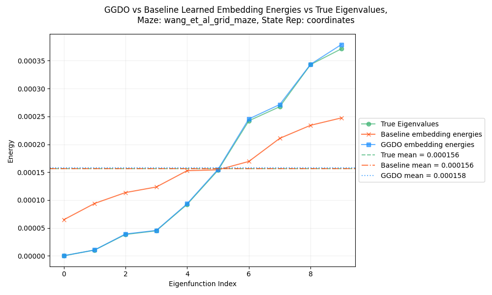
Hot DOG those are close! You can see that as before, the mean energies for GT, the baseline, and GGDO are all functionally identical. And you can also see that the baseline method has a “squashed” set of energies, never getting as low as the GT. But the GGDO ones are almost exactly the same curve as the GT. Very cool!
There are some more results, where they use the embeddings to define GCRL rewards, like they did in the previous paper. Similarly to that post, I won’t do that part today. Maybe I’ll do it in the future.
Wrapping up, afterthoughts
Simple is good
Again, it’s cool how simple a fix is. This is almost the ideal thing: understanding the underlying math which lets you see an easy win that’s simple to implement and doesn’t slow anything down.
I don’t know how generalizable this theme will be, but I’ll certainly be looking for it in the future. Like I said above, I was literally trying to solve this same problem, but via another constraint penalty term in the objective. They instead just changed the original objective to make it want to find this solution. Maybe it’s rare that that’s possible, but it’s still a cool idea.
Do they sort the baseline functions by energy?
One thing occurred to me. When they compare their method to the GT and baseline, for example:
are they sorting the baseline functions by energy? I.e., when I showed those plots of the learned vs true function energies above, I’m sorting the Baseline energies in ascending order, because if you don’t do that, they’re in some random order and harder to compare.
I ask because if they sort them, the SimGT and SimRUN results would prob be a lot better. For example, from looking at the figure above, the Baseline functions definitely aren’t finding the actual eigenfunctions, but if you squint, some of their functions definitely look kind of similar to GT ones for other dims. So if you matched those up with the closer GT ones, they’d prob have a better score (provided the energies are actually similar, which they might not be).
I suppose one argument against that is that in general, we can only approximate the energy for one of the embedding dim functions, so we can’t easily sort the baseline ones from smallest to largest energy, and it’s therefore a fair comparison to score them “as they come”. In contrast, for the GGDO ones, you know the first one is lowest energy, etc. But on the flip side, if we plan to use all of the embeddings as a set, then it might not matter what order they’re in, just that they’re finding the correct set. Maybe I’ll try this one day if I have the time.
Clear is good
I liked how (mostly) clear this paper was. A lot clearer in terms of experimental details than the predecessor paper. It’s really easy for them to just put a couple paragraphs in the appendix that can save a lot of time for anyone trying it.
That said, a few things could’ve been a bit clearer:
- they make the continuous mazes with PyBullet. It’s easy enough to see which cells are filled/etc for the discrete mazes, but the continuous ones are more ambiguous, given that the agent is a ball with diameter $1$ and the env is doing stuff with physical collisions. I wasn’t sure how wide the doorways should be (they say the width of “corridors” in the
PointMazeenv is $2$, so that’s what I used forPointRoom) - similarly, for the continuous action, they say:
- “For both environments, a ball with diameter $1$ is controlled to navigate in the environment. It takes a continuous action (within range $[0, 2\pi]$) to decide the direction and then move a small step forward along this direction.”
- Why couldn’t they just say what number that small step is?
- They don’t say which state rep they’re using for some of the discrete maze figures. Not a huge deal, but it’d take about 2 words to say.
- Super minor, but they say “$\textrm{SimRUN}(l, m)$ is in the range $[0, 1]$, and larger value implies larger inconsistency in the learned representations between $2$ runs”. I’m pretty sure that should be “consistency”.
And lastly: for the discrete mazes, we can just calculate the GT eigenfunctions by constructing the whole adjacency matrix/etc. For the continuous mazes, the state space is continuous so you can’t do that. They say:
For environments with continuous state spaces … the ground-truth representations (i.e., eigenfunctions) are approximated by the finite difference method with 5-point stencil (Peter & Lutz, 2003).
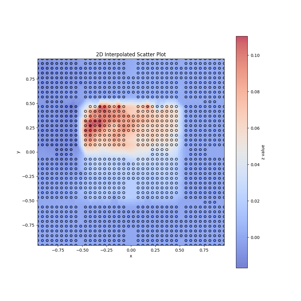
The reference is a textbook. I mean, I know the basic idea of a finite difference method, and there’s a Wiki article on it, but it’d still be nicer to have an appendix paragraph saying how they did it. I banged my head against the wall for a while, trying to discretize the free space of the continuous mazes into a finite set of discrete states, so I could use the discrete Laplacian approach, but it just wasn’t fully working. I kept getting obviously wrong eigenfunctions like this:
 Eventually I got a stencil-ish version working, and I guess it must work well enough (compare the GT for mine vs their Figure 4), but eh. I suspect my crappier results for
 PointRoom are at least partly due to me having to guess about some of these things with it. It’s my one result that’s different than theirs, but I think it’d be silly to spend too much time trying to get it to match, given the number of unknowns.
“Chasing figures” is a waste of time
When I try to implement one of these papers, one of the things I try to do to verify that I’ve understood it and implemented things right is reproduce the figures and any results I’m interested in. However, I def have a tendency to get tunnel vision and go way too hard on making my figures look as close to theirs as possible. For example, sometimes I’ll be frantically trying a ton of variations to get my figure looking just like theirs, and it’s not working, and I spend half an hour on it.
I think it’s partly because the feedback loop of updating and having a picture refresh and look better is very pleasing and addicting, but this post made me realize that beyond getting the basics of the figure, it’s a waste of time, because A) who cares, this is literally a blog post, and B) more importantly, plotting software is insane and even slight differences or mistakes they (or I!) might’ve made can change the look of a plot.