The dogtail party problem: ICA and blind source separation
Background
Many of my neighbors have dogs. Sometimes, a conversation will start between them, where one dog starts barking about something, a dog in a different house responds while the first one is still barking, and then another starts, and another, and soon enough $N$ dogs are barking at the same time.
My dog Goose is the silent type, but her ears perk up and you can tell she’s interested in hearing what they have to say… but they’re all barking at the same time. You can see her thinking, you fools! Bark one at a time. All your barks are mixing together and I can’t understand what you’re saying about that intriguing scent you smelled the other day!
Poor Goose, she’d never know what the deal was with that smell. However, one day, she had a stroke of inspiration: if she could coordinate with $N - 1$ other dogs she knows in the neighborhood, and they each recorded the mixed barks they were hearing, and met up later to compare them… maybe they could figure out what the original barks were?
Let’s see how!
Some setup and notation
We write each source signal (one dog barking) as a random variable (RV) $s_i$, and then write all the source signals together as a random vector of original signals $s = [s_1, s_2, \dots, s_N]$. We make a few reasonable assumptions:
- None of the $s_i$ have a Gaussian distribution
- All the $s_i$ are independent from each other
Then, we call Goose and her buddies the $N$ “receivers” of the source signals. Each of them is still getting some confusing mix of the source signals. However, because they’re in different houses, each of them gets a different mix of the source signals. We call each of the receivers mixed signals $x_i$, and the vector of all of them $x$. We make a few reasonable assumptions about them:
- The source signals combine linearly at each receiver
- We ignore phase shifts that would definitely occur due to the sources traveling different distances
If the sources are audio sources like different dogs barking, then each of the $s_i$ (and $x_i$) are actually time varying signals $s_i(t)$, but we’ll ignore the time dependence here (but we’re definitely leaving information on the table by doing that!). We’ll just treat each as RV with some distribution.
Since the source signals get mixed linearly at each receiver, if we call the square mixing matrix $A$, we have $x = As$. If we say $W = A^{-1}$, then $s = W x$, so if we could find $W$, we can get the original signals.
But how will Goose and co do this?
The high level strategy
Here’s the high level idea and strategy:
- We consider a single row $w_i$ of the matrix $W$ in $s = Wx$, and define a scalar $y_i = w_i \cdot x$
- By some arithmetic, we show that this is equal to a linear sum (determined by the value of $w_i$) of the source signals
- The Central Limit Theorem (CLT) tells us that the distribution of a sum of $M$ independent RV’s approaches a Gaussian, in the limit as $M \rightarrow \infty$
- If the value of $w_i$ is such that $y_i$ is a sum of the different independent $s_i$, then via the CLT, the distribution of $y_i$ would be closer to Gaussian
- On the other hand, if the value of $w_i$ is such that this linear sum is actually equal to a single one of the source signals, $y_i = s_j$, then it will be non-Gaussian (NG), as we assumed of the source signals
- Therefore, we want to find the $w_i$ that maximizes non-Gaussianity (NG) of the distribution of $y_i$
- To do this, we instead maximize (with respect to $w_i$) a proxy function $J(w_i)$ of the NG of $y_i$
- If we naively repeated this process, it’d give us the same $w_i$ every time. Therefore, to get the $w_j$ for the next source, we have to remove the projections of the current $w_j$ onto the previously found $w_i$ during each step of its optimization
This problem is of course the “cocktail party problem” among a bunch of other names, and the strategy above is known as Independent Component Analysis (ICA). And I’m basically just rehashing what they explain in “Independent Component Analysis: Algorithms and Applications” by Hyvärinen and Oja. Despite there being a few typos, unnecessary details, and ambiguities, it’s actually pretty well explained and readable. The algorithm itself is called the FastICA algorithm, though there are many variants and ways to do the same thing.
Motivating non-Gaussianity
Here’s a diagram I made of the main idea, that I found helpful:
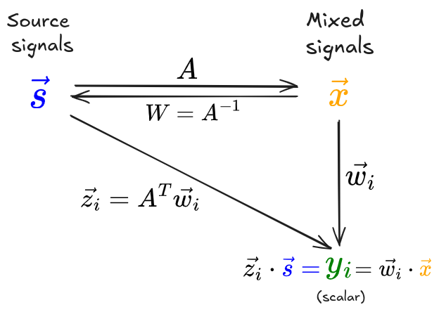
(I’m glossing over an important detail in the diagram: usually we preprocess the mixed signals by doing an eigendecomposition of their covariance matrix, $\mathbb E[X X^T] = E D E^T$; this gives a decorrelated data matrix $\tilde X = E D^{-1/2} E^T X$, which is actually what we use going forward. So technically $W$ isn’t the inverse of $A$, but the inverse of $\tilde A = E D^{-1/2} E^T A$.)
$w_i$ is a vector we’re considering, one row of $W$ (they have the vector symbols in the figure but I’m gonna drop them going forward). We start with the expression $y_i = w_i \cdot x$. We massage this by plugging in $x = As$ to get $y_i = w_i \cdot (A s)$. Then, if we define the vector $z_i = A^T w_i$, and plug that in, we get $y_i = w_i \cdot (A s) = z_i \cdot s$.
Like I mentioned in the high level strategy, $y_i = z_i \cdot s$ is a linear sum of the source components. This is conceptually useful, because the source components are independent and therefore the CLT tells us how the distribution of $y_i$ will behave (in terms of being Gaussian vs NG) for different possible $z_i$ values:
- If $z_i$ is one-hot on $j$th component –> $y_i = s_j$, and therefore $y_i$ is non Gaussian (as we assumed for the sources)
- If $z_i$ is uniform across its components –> $y_i$ is a sum of independent RVs, and therefore more Gaussian
Unfortunately, we don’t have either $z_i$ or $s$, but we have the equality that \(y_i = z_i \cdot s = w_i \cdot x\) and we do have $w_i$ and $x$. So, we can choose a $w_i$ vector, combine it with the mixed signals $x$, and then look at the distribution of $y_i$ for that $w_i$. We want to find $w_i$ such that $y_i$ distribution is as NG as possible. But how?
Estimating non-Gaussianity
There are a bunch of ways you can do this. Kurtosis is a measure of how “fat” or “skinny” the tails of a distribution are compared to a Gaussian, so you could do that. However, supposedly this is very sensitive to outliers so it’s not preferred.
A better way is by using negentropy. To briefly explain it: the entropy of a distribution increases with higher variance. But if you fix the variance to some value and consider any distribution with that variance, then a Gaussian distribution has the maximum entropy possible for that fixed variance.
Therefore, for a fixed variance, a very low entropy distribution would be non-Gaussian. Negentropy is basically just subtracting the entropy of the distribution from the entropy of a Gaussian with the same variance: $J(y) = H(y_G) - H(y)$. Since $H(y_G)$ is the most entropy it can have with that variance, $J(y)$ will be zero when $y$ is Gaussian, and positive the more NG it is.
Finally, estimating negentropy can be hard, so they give this magic approximation for it: \(J(y) \approx \bigg[ \mathbb E[G(y)] - \mathbb E[G(\nu)] \bigg]^2\) where $\nu$ is a standardized Gaussian RV and $G$ is “practically any non-quadratic function”, but they give a couple “very useful” choices, like this one: \(G_1(u) = \frac{1}{a} \log \cosh (a \cdot u)\) where $1 \leq a \leq 2$. Note that part of what makes this approximation convenient is that we don’t have to discretize or model the distribution’s density in any way, we simply do it from samples.
Here’s a little figure I made to illustrate:
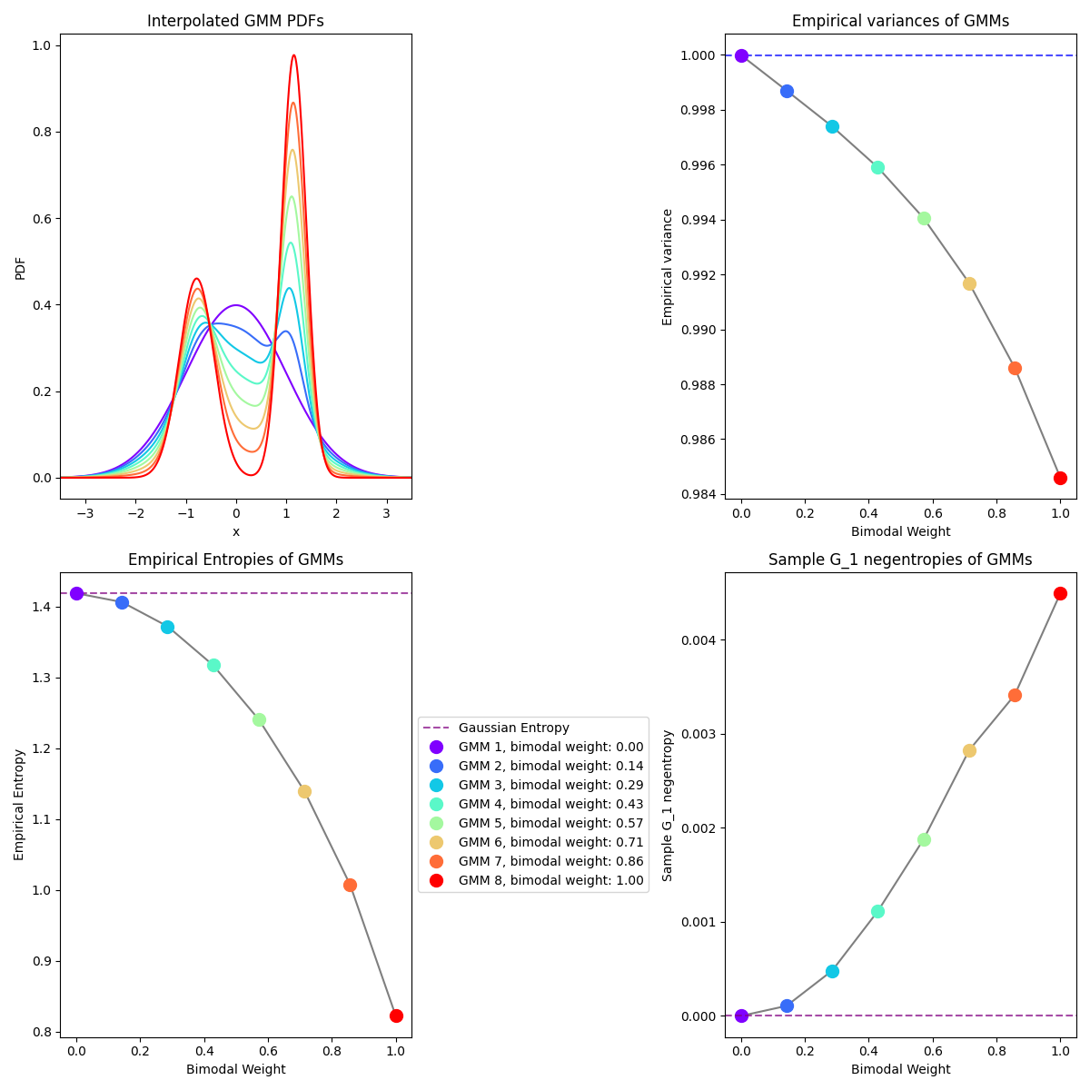
In the upper left plot, the purple curve is a standard Gaussian distribution, and the red curve is a bimodal, obviously very NG distribution. The other curves are distributions that are interpolating smoothly in between the Gaussian and bimodal one, so we can see how the properties change. I adjusted the means of the interpolated ones such that their variance is very close to one, like the unit Gaussian (as you can see in the upper right plot).
In the lower left plot, you can see an empirical entropy of each distribution (calculated by just discretizing the curve and summing). As expected, the Gaussian has the highest entropy, and the less Gaussian the distributions get, the lower entropy they have (for about the same variance).
Finally, in the lower right, I’ve calculated the negentropy using the approximation above – you can see it grows, the less Gaussian they get.
Full process
That’s almost all of it, and the important part anyway. There are really two remaining parts I’m going to gloss over.
Recall that for $N$ sources/mixed signals, we want to find $N$ vectors $w_i$ that will each give back one of the mixed signals $s_i$. As I mentioned above, in the FastICA algorithm, we find them one at a time, each one being optimized in an iterative loop until it converges.
As above, a given $w_i$ value gives rise to the negentropy approximation $J(w_i)$. The update we do to $w_i$ in each iteration is basically a Newton step that’s maximizing $J(w_i)$ subject to the constraint that $|w_i|^2 = 1$. They use another clever approximation to derive the update form (you can see in the articles above), but I don’t think this is super important; the key point is just we do the constrained optimization on the negentropy objective.
The other part is that for each $w_i$, we initialize it with a random (unit norm) vector. However, if we naively just did the same thing for each $w_i$, the optimization would always converge to the same fixed point! Therefore, to make sure we get different $w_i$, in each iteration of the optimization for the current $w_j$, after doing an update, we project it onto the previous $w_i$ we’ve found, and subtract those projections. This ensures that only the perpendicular component remains, and it’ll find the remaining different $w_j$. The result is that $W$ will be an orthogonal matrix.
Experiments
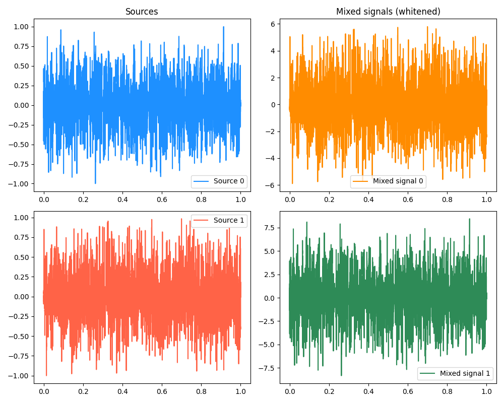
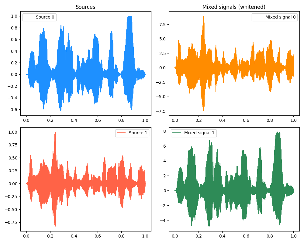
First, here’s a simple example with two sources. We can look at some plots of the original sources, as well as the mixed signals:
Then, we can look run the process described above. Just this once (as a treat), I’ll plot the values of $w_i$ and the objective $J(w_i)$ during the optimization process:
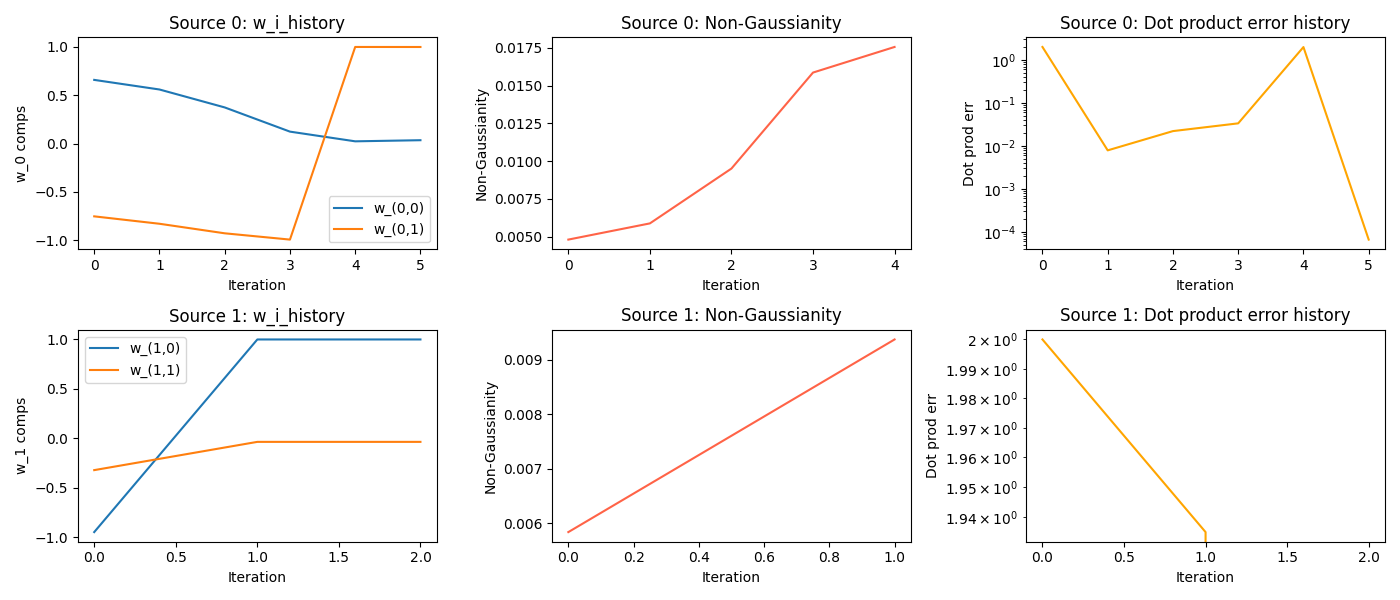
You can see:
- $w_0$ takes ~5 iterations to converge, and then $w_1$ converges way faster (1st column)
- I think this is because when it subtracts its projection onto $w_0$, it’s only in 2D, so that basically solves it?
- the $y_i$ distributions get more NG (2nd column)
- the iteration ends when the dot product between $w_i$ iterates doesn’t change below some threshold in subsequent steps (3rd column)
Finally, once we have all of the $w_i$, we can calculate the original sources!
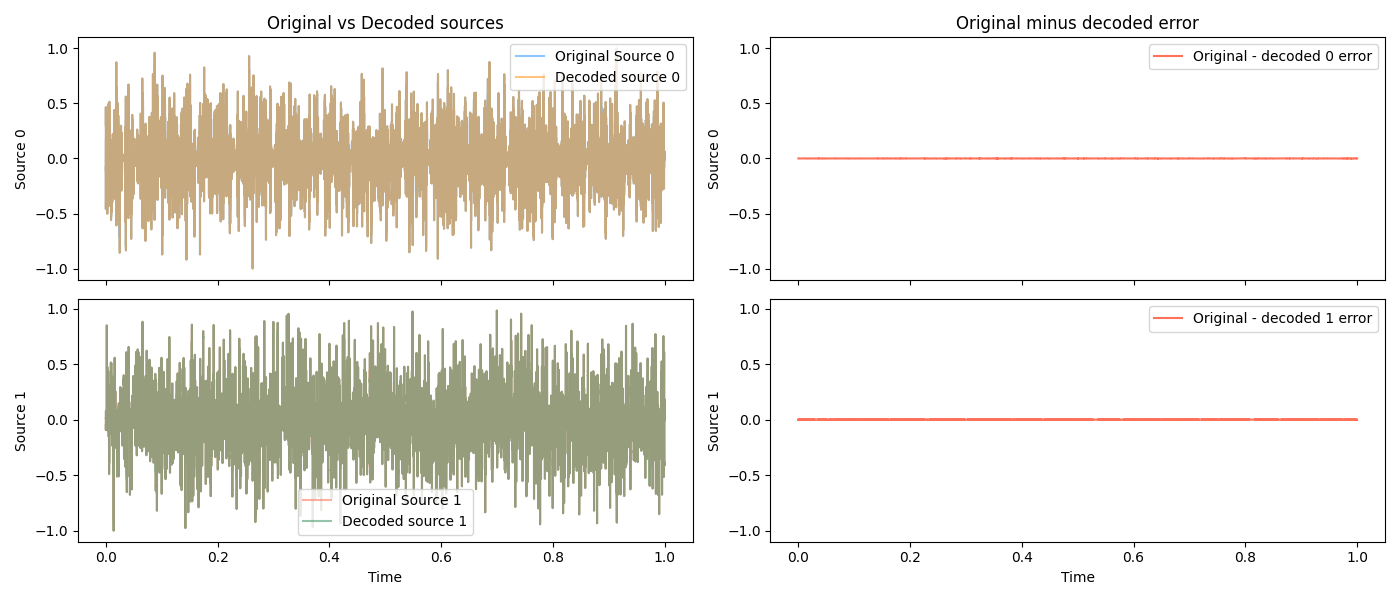
Zoomed in on a few locations, so you can see how well it’s matching:
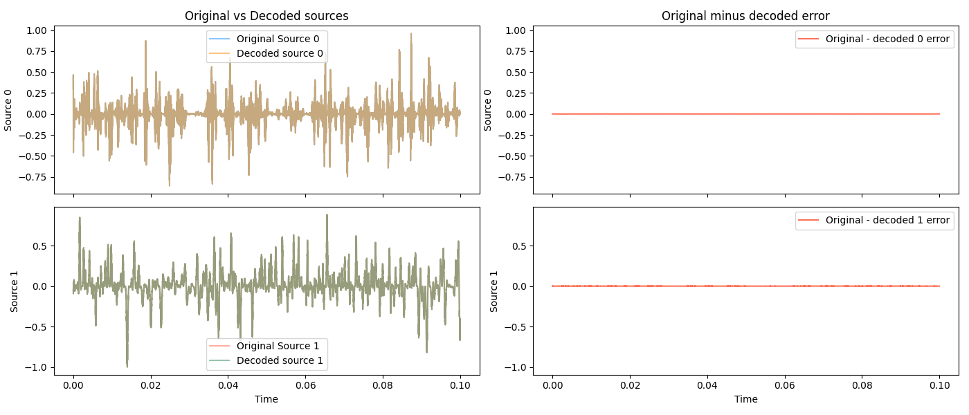

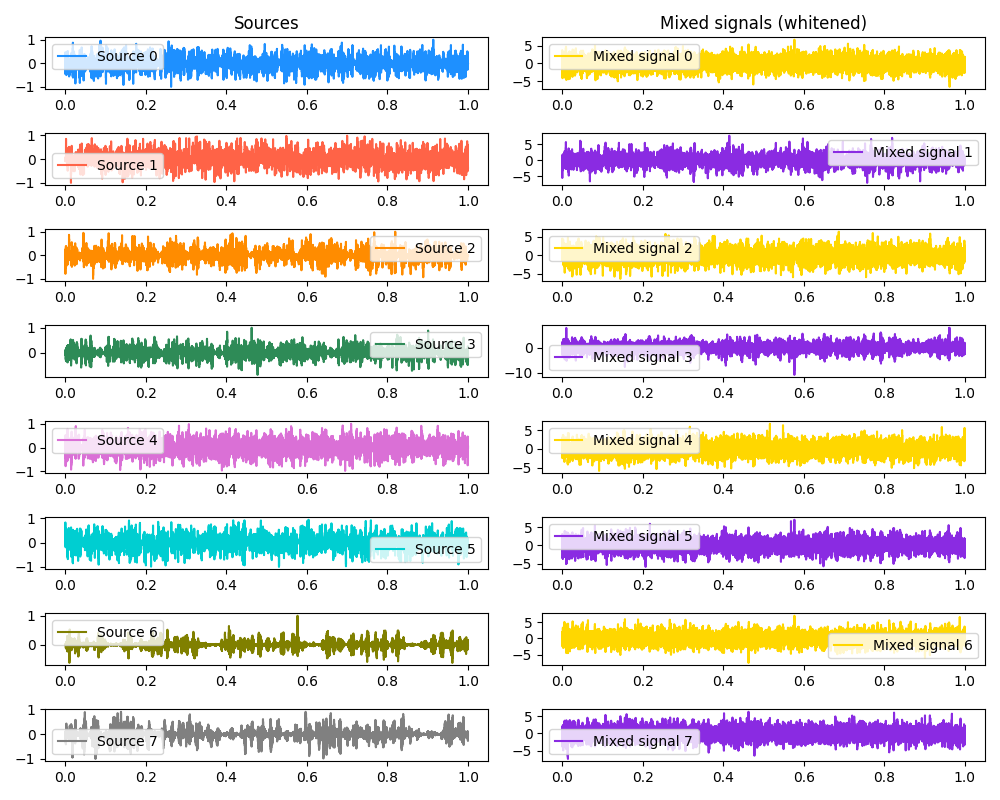
Two sources is easy, though. What about… eight dogs!?
Original and mixed:
And some decoded at different scales:

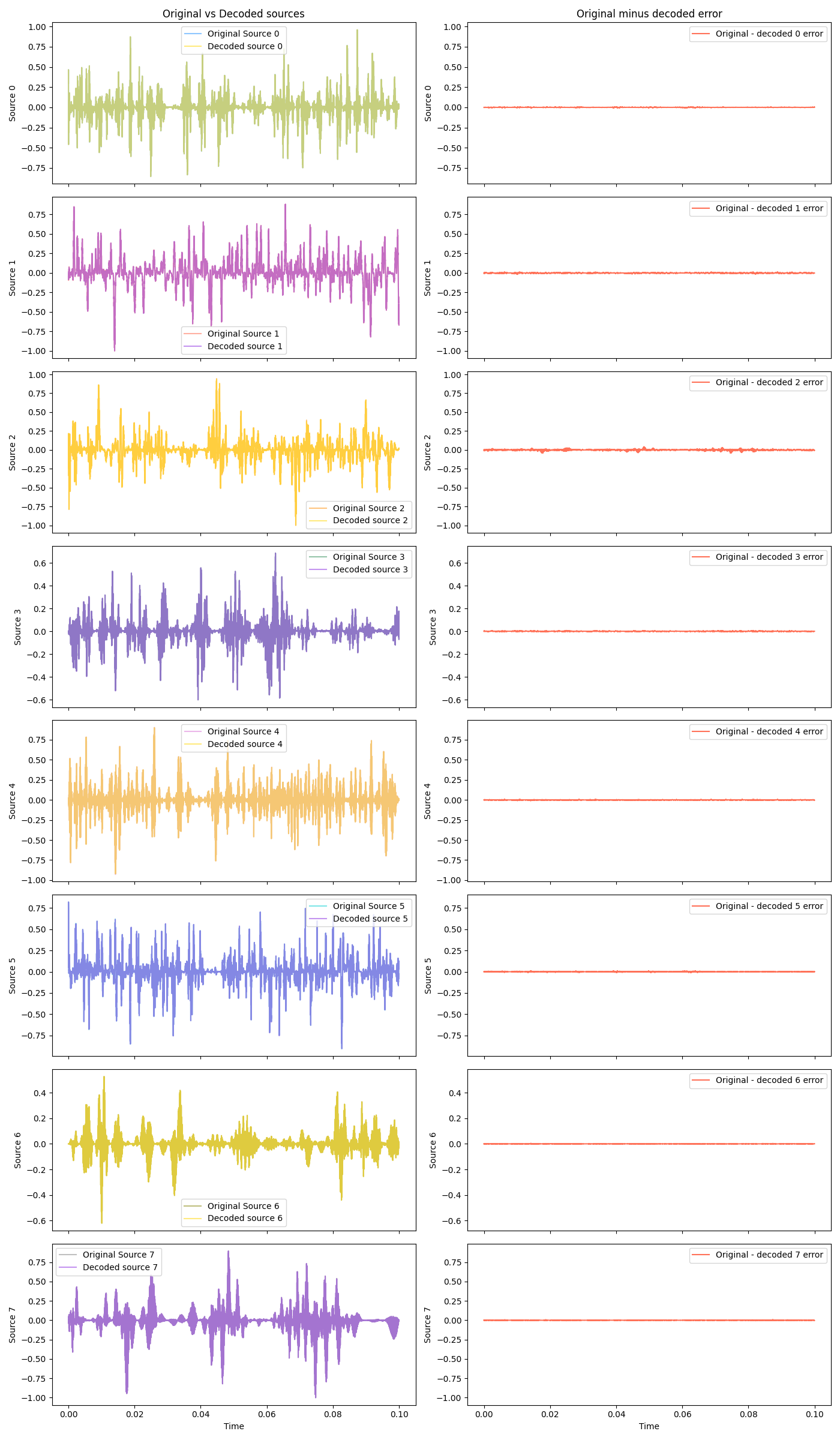
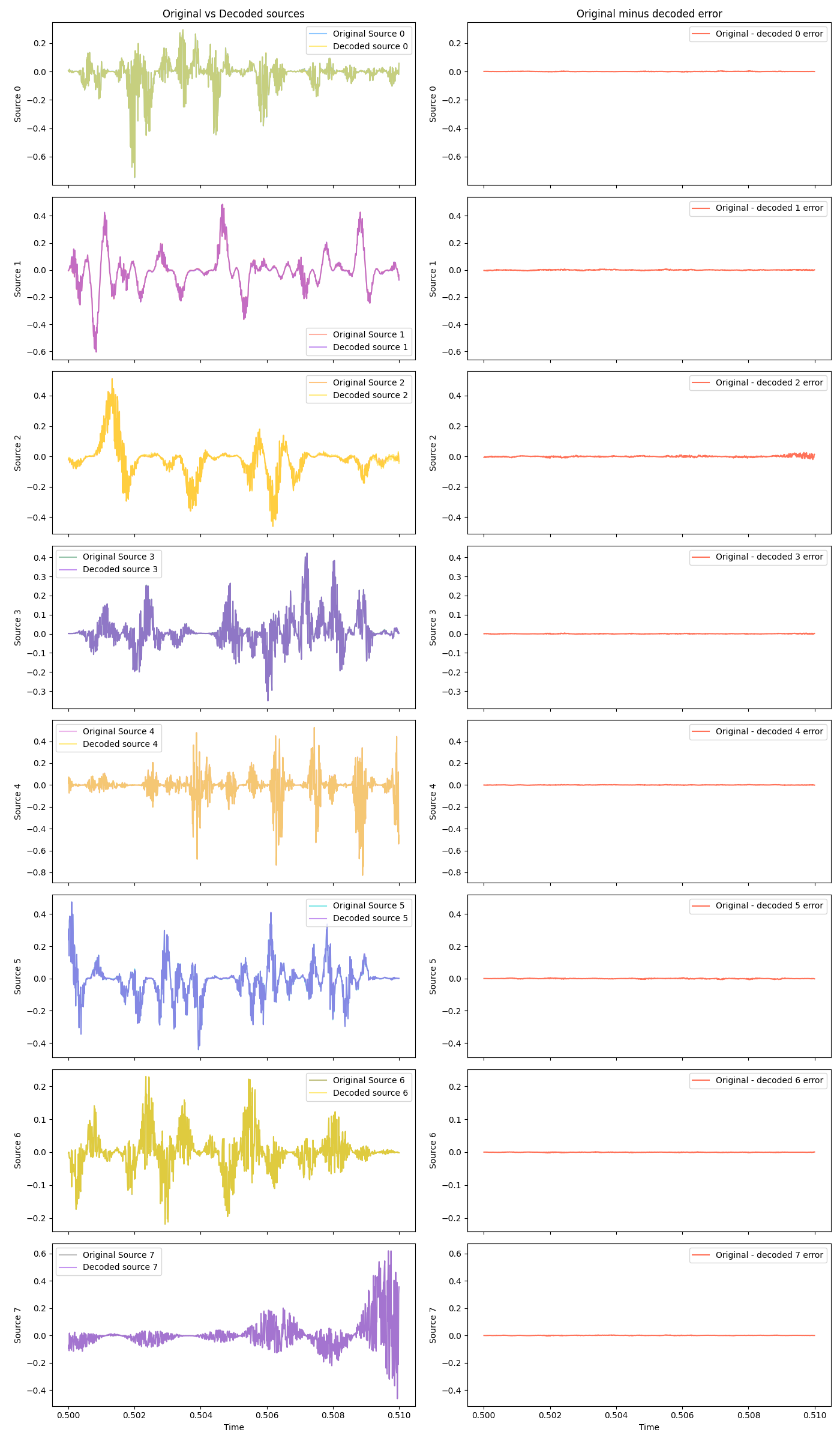
Hot damn! They basically overlap so much you can tell them apart, without zooming waaay in.
Real audio sources
Okay, enough fooling around. I promised you a dogtail party and a dogtail party you shall get. Doing it with “synthetic” signals I made myself is one thing, but does it work with real audio signals?
Below are eight 2.5 second clips, the original sources. For added fun, don’t listen to them yet, and instead skip down to the mixed signals! See what you can pick out from the voices in the party.
Then we mix them. Here you can see the original source and mixed signals:
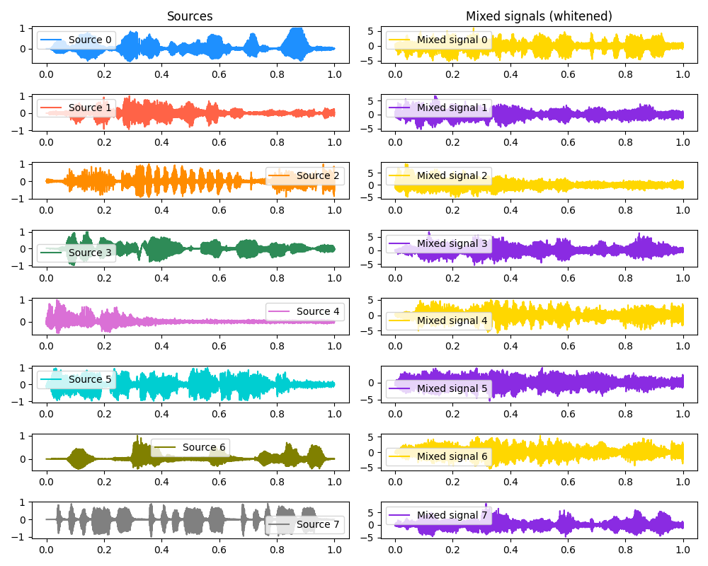
And here are the mixed signals:
Give a couple of them a listen, it’s absolute chaos!
How does the algo do on these? Same plots as before, same scales:


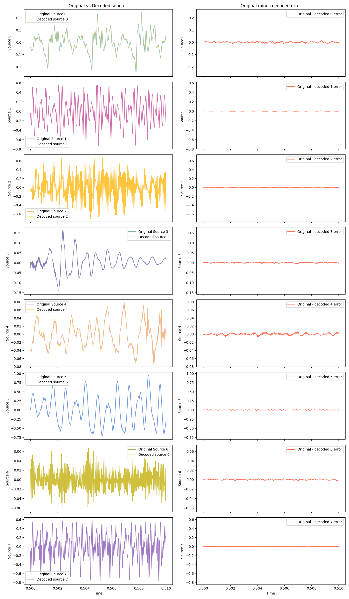
It absolutely nails it! Here are the decoded signals:
One last experiment, because this surprised me a lot (I’m still wondering if I just messed something up). Those audio signals above are pretty different from each other; wildly different sounds and voices. However, when I was originally choosing the audio clips from random stuff I found online, I found a sample of some spoken word poetry (which source 0 in the one above came from). It was pretty long, so I thought I’d just clip sections from it and use them as the different sources.
Since these were from the same recording, they’re of the same speaker. Here are just two of them:
and their waveforms:
you can see that the voice sounds the same, but the waveforms do look pretty different from a high level at least. And a scatter plot of them and an estimate of their mutual information (see more below) indicates that they’re pretty independent:
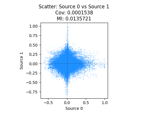
and there are only two signals! So I thought this shouldn’t be too hard. Here’s what the mixed signals sound like:
I think I can even tell them apart, after a few listens. But, decoding it does terribly:
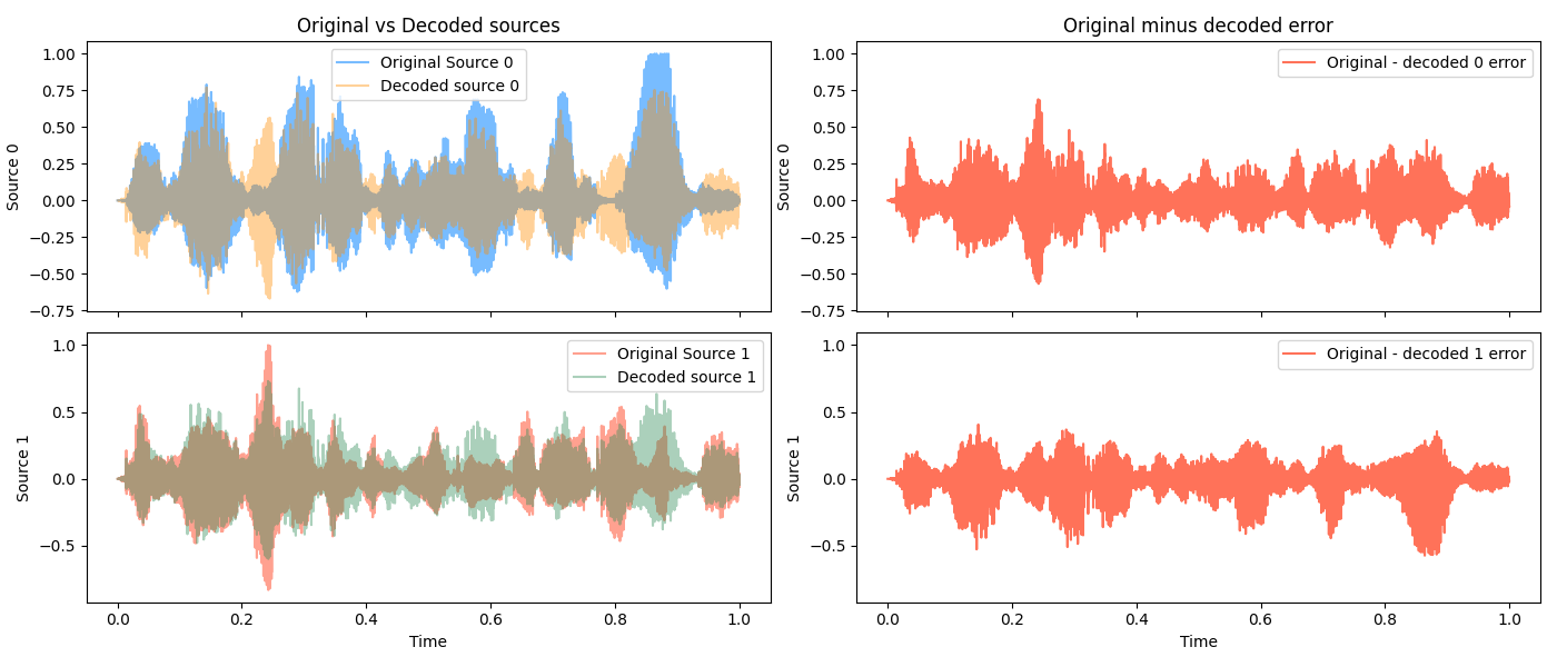
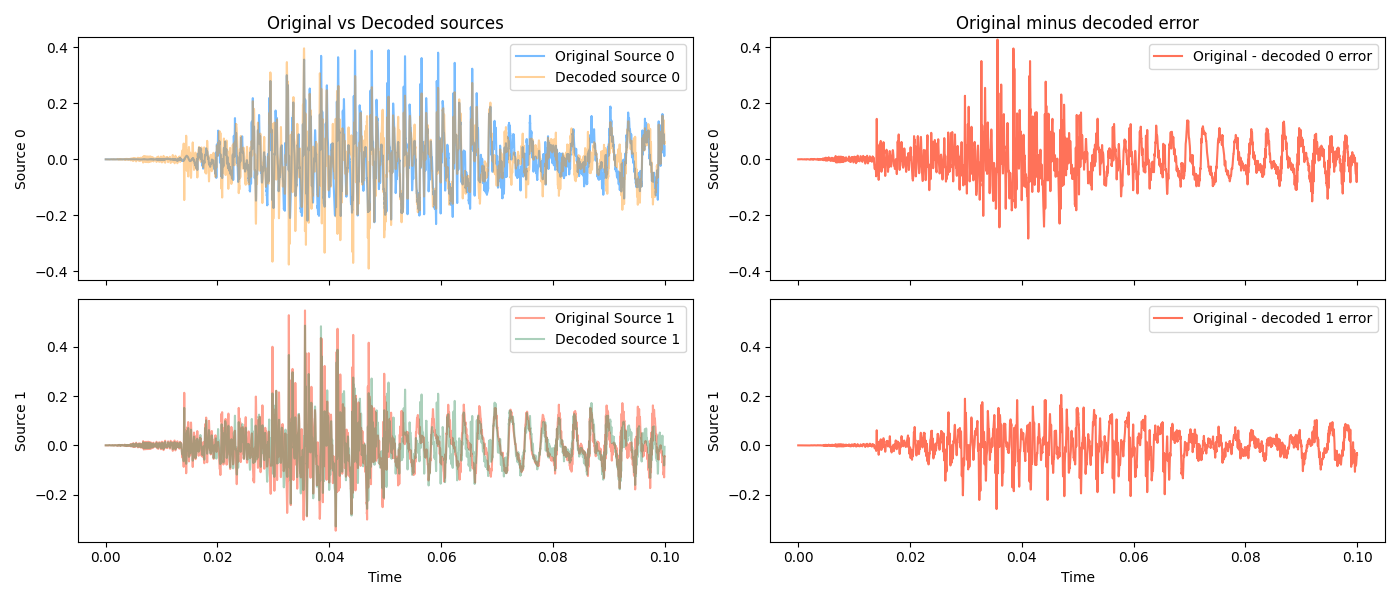
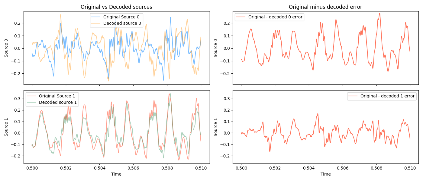
and this is reflected in how the decoded signals sound:
On one hand, this makes intuitive sense. It’s way harder to distinguish the same voice layered than different voices.
On the other hand, it seems very likely to me that our auditory system is using something more like the spectrum of sounds to do this, and recall that here, the algorithm actually has no sense of “time”; the signals are just joint distributions.
And further, I’m not sure why this is failing, really. The signals are as non-Gaussian as any of the ones above, and I showed some evidence above for them sure looking pretty independent (the scatter plot and MI are about in line with the successful experiment).
If I wave my hands and take a guess, my guess is that due to the voice being the same, certain important frequencies are “aligning” and making it a lot less independent for many of the samples. That said, I don’t have a good answer for why that isn’t shown more in the scatter plot/MI.
Discussion
Why do we need this fancy method for estimating the (neg)entropy?
Above I showed their approximation to the negentropy $J(y)$, that they optimize to maximize NG. They say
The problem in using negentropy is, however, that it is computationally very difficult. Estimating negentropy using the definition would require an estimate (possibly nonparametric) of the pdf.
And, yeah, usually finding a PDF is something you want to avoid if possible. The usual reason for this that comes to mind is that when the support of the distribution is high dimensional, it makes modeling harder and means integrating over volumes will be intractable.
However, here, the support is the scalar $y$, right? And typically the data $x$ is whitened, so we have a good sense of its range. It seems like it’d actually be pretty feasible to just bin $y_i$, get a categorical distribution, and calculate an empirical entropy, and use that to update $w_i$.
I’m probably missing something here. I guess one thing could be the update step. We’d like to take the gradient with respect to $w_i$ (as they do for the approximation), and maybe the binning of the $y_i$ samples would mess that up. You could definitely do a gradient-free CMA-ES hill climbing strategy, but gradients are really nice as the dimension (in this case, of $w_i$, i.e., the number of sources) gets higher.
Producing independent time series data that’s also non Gaussian is actually kind of hard?
If you recall, two assumptions you have to make about the source signals are that A) they’re independent, and B) they’re non-Gaussian. I wanted to make some fake but plausible audio looking signals to use as the source signals, but I found that it was actually pretty hard to make some time series data that satisfy both of these! I was basically adding up a bunch of square and sine waves with frequency and amplitude modulation, plus some random noise.
I think I might actually do a separate post on this in the future because it’s pretty interesting, so I’ll just show a couple examples here.
To check how independent the distributions of the source signals are, I’m binning all the $(s_1, s_2)$ pairs to form a discrete 2D joint PDF, and then calculating the empirical mutual information ($I(S_1; S_2)$) of them. Higher $I$ means less independent, and truly independent distributions would have $I(S_1; S_2) = 0$.
To check how non-Gaussian each source signal is on its own, I’m mostly just plotting it with the closest Gaussian fit to its histogram. But, since I have it anyway, I can calculate the non-Gaussianity measures we used above.
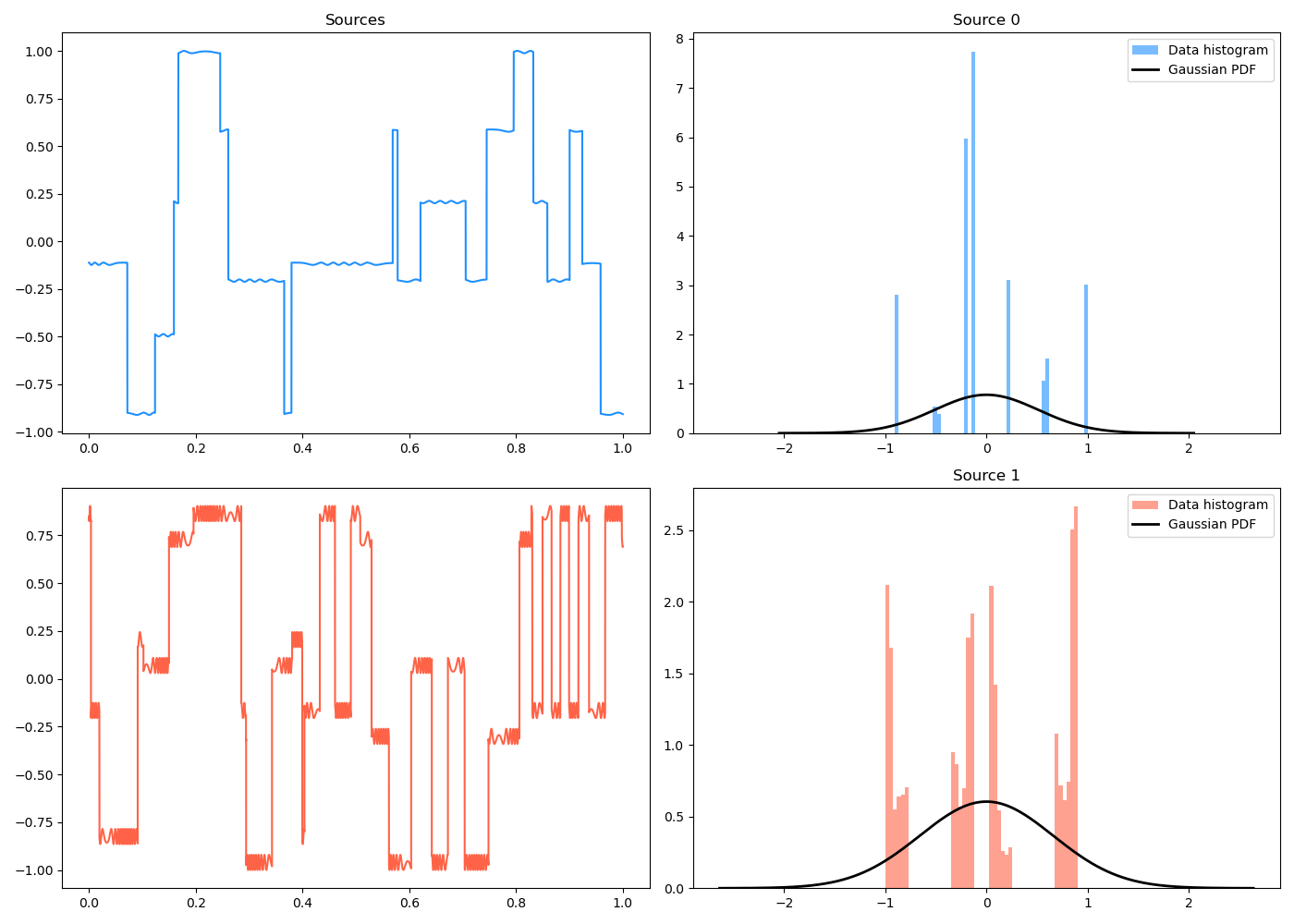
Here’s an example of two source signals that you can see are definitely pretty non-Gaussian from their histograms:
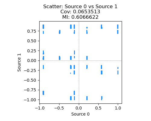
However, if you plot a scatter plot of them, you can see that the MI is $I(S_1; S_2) \approx 0.6$ and it’s just clearly not independent – for example, if you know $s_1 = 1.0$, $s_2$ has a very different distribution than if $s_1 = -1$.
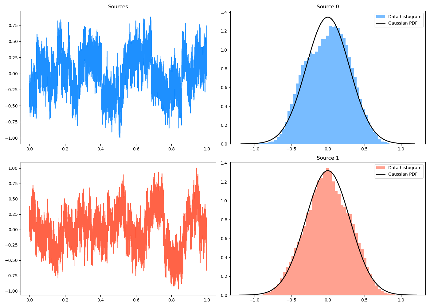
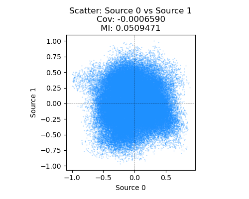
On the flip side, here’s another pair of source signals. You can see (next plot) that their MI is much smaller and their scatter plot looks like a pretty symmetric cloud, but their histograms now look pretty darn close to Gaussians. Ruh roh!
Brainstorming and ideas
I’m trying to get in the habit of ending these explorations with some brief brainstorming.
(If I have a direct application I’m learning a topic for, then it’s already easily concrete. But often I’m just learning an approach for general interest, with the hope that maybe someday in the future I’ll pattern match it to a problem I’m facing and realize it’s useful for solving it. However, I think a better idea would be to instead actively try to crystallize it by forcing myself to come up with ideas, even if they’re dumb.)
So I want to consider two aspects: A) concrete, direct applications of the method (e.g., could you apply ICA to problem X?), and B) more thematic takeaways. So…
Direct applications
I’m really reaching here, but that’s the point. So I’m searching for things where some (unknown) signals (with some constraints) get mixed in a linear (unknown) way, and I just get the results of them. I have a hammer, so let’s desperately look for some nails.
I guess one we could consider is a Markov transition matrix $P(s’ \mid s)$, applied to a state distribution $\rho(s)$ (let’s assume the policy has been “baked in” as is often done, so $\pi(a \mid s)$ gets combined with $P(s’ \mid s, a)$ to just get $P_\pi(s’ \mid s)$ and I’ll drop the subscript). $\rho(s) = \rho$ is a density over all the states in the MDP (a vector if there are a finite number of states), and $P(s’ \mid s)$ “mixes” them to the state distribution in the next timestep, $\rho(s’) = \rho’$. In matrix notation, this is $\rho’ = P \rho$. Super naively, we could imagine getting measurements $\rho’$ (itself typically infeasible but… just be cool ok?), but not knowing $P$ or $\rho$, and using ICA to figure out $\rho$ and then $P$.
But I suspect this wouldn’t work because of problems with source independence (among many other problems). For example, if we were given a big compilation of a bunch of trajectories in the MDP, the $s’$ of one transition would be the $s$ for another transition, and then it seems like the sources would definitely not be independent.
Another one I was thinking of is the case where the scalar reward the agent receives is actually the linear sum of several reward terms $r_j$, i.e., $R(s, a) = \sum_j w_j r_j(s, a)$. Let’s just consider it for a single $(s, a)$ pair for now, and write the sum in terms of a vector dot product, so we have $R = w \cdot r$. However, it’s common to set up different “tasks” that are defined by different $w$ weight vectors, so let’s call each one $w_i$, and then $R_i = w_i \cdot r$. Then, across the different $i$ used, we’d have $R = W r$, where $R$ and $r$ are vectors and $W$ is the matrix with the $w_i$ forming its rows. This kind of has the form of the BSS problem, where (for a single $(s, a)$) the agent would receive different $R_i$ signals depending on the different $w_i$ that was being used. We could then think of applying ICA to recover the reward components $r_j$ as well as all the weight vectors $w_i$.
The reason this idea doesn’t seem very interesting is that usually when this is done, the algo designers give the $w_i$ as inputs to the models and also have specified the $r_j$ themselves. So I’m not sure if there’s actually any need for this.
Thematic takeaways
ICA feels a little like magic to me: I think if someone described the problem to me and I didn’t know of the method, I might say that it’s impossible. “What do you mean, you just have the mixed signals but you don’t know anything about the source signals or how they were mixed? They could be anything!”
One interesting thing is that although the problem is often posed as $x = As$ and we want to “unscramble” $x$ to get $s$, we’re not actually after the particular $s$ at all; after we solve $x = As$, we have the mixing matrix $A$ which is the more general solution and will mix any other future signals the same way.
Related to this is something interesting about the info we have and what we solve for. If we write a typical supervised learning problem in which we have (feature, label) pairs $(x_i, y_i)$ and learn a model $y = f(x)$, then you can write the input/transform/output as: \(x \overset{f}\rightarrow y\) and the BSS problem as: \(s \overset{A} \rightarrow x\) The interesting thing is that in the SL problem, we have $x$ and $y$ and have to figure out $f$, the missing third leg of the stool. In the BSS problem, we only have $x$ and have to figure out both $s$ and $A$! That’s pretty weird and would feel almost nonsensical in the context of the SL problem. So I guess one thematic takeaway is that sometimes, certain constraints/assumptions (i.e., the linear mixing, NG of the source signals, etc) can make an otherwise impossible problem very solvable.
One last theme that I’ll need to look out for in the future is the move with the CLT that lets this whole method work. From a high level, it’s kind of saying:
“the CLT tells us that if A (some RV is a sum of multiple independent RV’s), then B (that RV will be more Gaussian). Therefore, if we intentionally search for not B (a sum RV with a NG distribution), then not A (the RV must be composed of only a single RV)”
I.e., using the contrapositive of the CLT. Using the contrapositive is classic proof stuff, but I feel like I haven’t seen it used as much for actual methods (I’m sure there are countless examples, I just don’t know them), and more specifically, using a statistical version of it.
Welp, that was more than I expected. Anyway, as usual, let me know if I’ve made any mistakes or missed anything!