Keep your eyes on the prize: offline GCRL with OGBench
Previously, I implemented IQL, an offline RL algorithm. My main motivation there was to have a nice, simple, stable offline RL algorithm that I could use to learn from offline datasets, to experiment with some ideas in the future.
Today, I’m following up on the IQL paper with an implementation of a few of the algos implemented in OGBench.
OGBench?
Simply, OGBench is a large benchmark of offline GCRL (OGCRL) datasets and corresponding envs, with implementations of six common offline GCRL algos, and the code for all of it open sourced.
This might sound like yet another “here’s our new benchmark please use it!!” paper, but there’s actually way more to it than that. First, the datasets are thoughtfully designed to test several important challenges for OGCRL algos, with specific datasets targeting different challenges.
Second, the paper is super clear and unambiguous. Maybe it’s in my head, but when I read it I sense the frustration they have with previous attempts at doing this, that end up being ambiguous and difficult to use and no one ends up using.
Lastly, the algo implementations in the repo are written very simply and clearly! Despite it being written in JAX, which I’m not super familiar with, it was very clear. I can’t say how important that is if you have some practical question. That said, I barely needed it because the paper was written so cleanly.
which brings us to today
So, this is what OGBench is trying to do – make a really clear and reproducible benchmark that researchers can use to experiment with new OGCRL algos in a way they can trust the results of. For example, after finishing my IQL post last time, I was pretty sure I had done things right, but wasn’t 100% sure – I couldn’t reproduce some of their results given all the env/datasets mess. That was unsatisfying, so I wanted to do implement the algos in OGBench so I could be sure my setup is working well.
They implement six algos: GCBC, GCIVL, GCIQL, QRL, CRL, and HIQL. Today, I’ll just be implementing GCBC, GCIVL, and GCIQL, and I’ll do the others (which are cooler!) another time.
Anyway, since I had already implemented BC and IQL for the IQL post, this meant that it was actually pretty quick to put these three algos together.
Results up front
Today, instead of doing the usual thing where I ramble for six thousand words and then show some results at the end, I’m gonna flip the script and show results up front, and extended jabbering later. Let’s see some shiny results!
First a disclaimer: I didn’t run all environments, because there are a bazillion of them, and for now I mostly just want to verify that my algos are working right. So here’s what I did:
- I chose some subset of the datasets (10) that they reported decent to good scores for, for GCIVL and GCIQL
- I also did a couple of these for GCBC that it does decently on (it does pretty bad on most)
- while the paper ran each with 8 seeds, I just did one training run for each (aside from a few with extra copies from earlier test runs)
- aaaaaand sorry, but I’m not doing the pixel-based ones. Compute doesn’t grow on trees!
- For each run, I evaluated the final policy on 100 episodes, cycling between the different eval tasks
Here are the results. In each table entry, my results are the colored ones to the left, and the corresponding scores from the paper are in the parentheses (specifically their $\mu \pm \sigma$ across seeds):
\[\begin{array}{lrrr} \hline \text{dataset name} & \text{GCBC} & \text{GCIQL} & \text{GCIVL}\\ \hline \text{antmaze-medium-stitch-v0} & \textcolor{limegreen}{64}\ (45 \pm 11) & \textcolor{limegreen}{31}\ (29 \pm 6) & \textcolor{limegreen}{50}\ (44 \pm 6)\\ \text{antmaze-teleport-navigate-v0} & - & \textcolor{limegreen}{40}\ (35 \pm 5) & \textcolor{limegreen}{48}\ (39 \pm 3)\\ \text{antsoccer-arena-navigate-v0} & - & \textcolor{limegreen}{48}\ (50 \pm 2) & \textcolor{limegreen}{59}\ (47 \pm 3)\\ \text{cube-single-play-v0} & - & \textcolor{limegreen}{74}\ (68 \pm 6) & \textcolor{limegreen}{50}\ (53 \pm 4)\\ \text{humanoidmaze-medium-navigate-v0} & - & \textcolor{orange}{24}\ (27 \pm 2) & [\textcolor{limegreen}{39},\ \textcolor{limegreen}{25}]\ (21 \pm 2)\\ \text{pointmaze-large-navigate-v0} & \textcolor{limegreen}{34}\ (29 \pm 6) & \textcolor{red}{24}\ (34 \pm 3) & \textcolor{limegreen}{40}\ (45 \pm 5)\\ \text{pointmaze-medium-stitch-v0} & - & \textcolor{limegreen}{20}\ (21 \pm 9) & [\textcolor{orange}{54},\ \textcolor{limegreen}{60}]\ (70 \pm 14)\\ \text{pointmaze-teleport-navigate-v0} & - & \textcolor{limegreen}{28}\ (24 \pm 7) & \textcolor{red}{36}\ (45 \pm 3)\\ \text{puzzle-3x3-play-v0} & - & \textcolor{red}{87}\ (95 \pm 1) & \textcolor{limegreen}{7}\ (6 \pm 1)\\ \text{scene-play-v0} & - & \textcolor{limegreen}{53}\ (51 \pm 4) & \textcolor{limegreen}{48}\ (42 \pm 4)\\ \hline \end{array}\]For the ones I did multiple runs with, the results from the different runs are in square brackets. I’ve arbitrarily colored my results like so, if we call my score $S$:
- green: $S \geq \mu - \sigma$
- orange: $\mu - 2\sigma \leq S < \mu - \sigma$
- red: $S < \mu - 2\sigma$
You can see that most of them are pretty similar to the paper! And the only red ones aren’t terrible scores compared to their $\mu$ (24 vs 34, 36 vs 45, 87 vs 95), they just have pretty tight $\sigma$ for those ones, and my scores fall outside of them. If I look at those ones specifically, I can’t see anything that obviously indicates anything wrong with them, so my best guess is a combo of unlucky seed plus maybe very minor implementation differences. Looking at my training loss curves, they’re plausibly still slowly improving when I stop them at 1M steps, so if theirs learns a little faster for some reason, maybe that could explain it?
Anyway, enough of all this number talk! That’s not what you’re here for. You’re here to see videos of simulated robots do silly tasks!
Antmaze-medium, GCBC:
Antmaze-teleport, GCIVL:
Antsoccer-arena, GCIVL:
Cube-single, GCIQL:
Humanoidmaze-medium, GCIVL:
that’s painful to watch!
Pointmaze-large, GCBC:
Pointmaze-teleport, GCIVL:
Puzzle-3x3, GCIQL:
Scene, GCIQL:
These are all ones I cherry picked because they succeed at the task (although for some of them the majority succeed so I could just choose randomly).
Discussion, jibber jabber, blathering
The stochastic ones are deceptively bad!
Something they do in OGBench is define a small number of categories to divide the datasets up into. The categories challenge different aspects of OGCRL, so they’re useful for seeing which algos succeed or fail with respect to these challenges. One of those categories is stochasticity. Most of these envs are deterministic (I think), but they purposely built variants of pointmaze and antmaze (with the teleport suffix) that have “black holes” that randomly teleport the agent to a “white hole” if they enter it, to have some stochastic envs, as you can see in the video above.
Importantly, you can see that one of the black holes is in a dead end, so if it ends up there, the episode is a failure. Since a black hole has a 1/3 chance of failure and the agent can always succeed by just walking to the goal, optimal behavior means avoiding black holes entirely.
One interesting thing I noticed from watching the videos is the following. Looking at the teleport results I (and they) got in the table above, I got scores of 40/48 for antmaze-teleport-navigate and scores of 28/36 for pointmaze-teleport-navigate. These aren’t good scores by any means, but I don’t view them as total failures either. However, looking at a handful of the successful eval videos of GCIVL, antmaze-teleport:
All the teleport evals I’ve shown above are actually different “tasks”; there are 5 eval tasks for each env, which they show in this appendix figure:
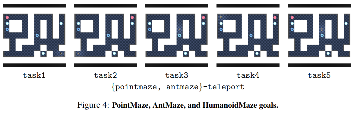
you can see that the goal (red dot) is only in two unique locations, but the ant starts in different locations depending on the task.
Watching these (successful!) eval vids definitely lowered my opinion of how much I think these algos “learned” the stochastic teleport envs. It really seems like it’s not avoiding the black holes, but rather making a beeline for them!
The thing is, there’s a white hole next to the goal for any of the tasks… so while going into a black hole has a 1/3 chance of immediate failure, it also has a 1/3 chance of putting the agent right by the goal! In the other 1/3 chance case, it resets it to a spot that’s far from the goal, but at least it gets to try again. So from the vids, I suspect that it’s found a local minimum in behavior where it can get an easy 1/3 success, at the cost of 1/3 failure.
In fact, if we assume that in the remaining 1/3 case it resets to exactly the original scenario, the chance of success turns into a geometric sum, adding up to $1/2$. The range $[1/3, 1/2] = [0.33, 0.5]$ is in fact the most that any of the methods (including the others I didn’t do in this post) achieve on any of the teleport datasets! So I highly suspect that:
- some algos don’t even learn to “use” the black holes and get very bad scores $< 1/3$
- the “good” ones learn to use black holes and get scores $\geq 1/3$ but $\leq 1/2$, and of these:
- some can steer better in that other $1/3$ case back to try again, and get closer to $1/2$
- while others can’t as well, and get closer to $1/3$
This could probably be shown more conclusively by changing the number of black/white holes, and the relative distances, such that it’s really clear when it is an optimal move (on average) to be going into a black hole, vs it being optimal to never go in them.
Stochastic category?
In their Results section, they have a Q&A style discussion. One of them says:
Q: Which methods are good at handling stochasticity?
A: For this, we can compare the performances on the large and teleport mazes in Table 2, where both have the same maze size, but only the latter involves stochastic transitions that incur risk. Table 2 shows that, value-only methods like HIQL and QRL (i.e., methods that do not have a separate Q function), which are optimistically biased in stochastic environments, struggle relatively more in stochastic teleport tasks. In contrast, CRL is generally robust to environment stochasticity, likely because it fits a Monte Carlo value function.
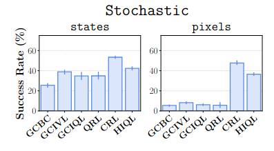
And, if we look at Figure 2, where they’ve broken down the results by dataset categories, this does appear to be right:
But… when I went to look at the results table (Table 2), it seems to clash with this:
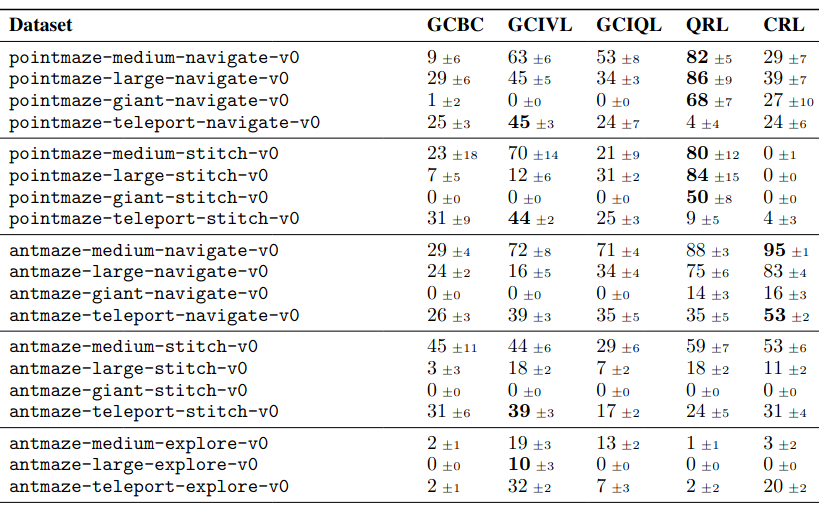
(I cropped out a bunch of datasets and the HIQL results here.)
Basically, if you look at the scores for the five datasets there that have teleport in their names, CRL is… not clearly winning? It only slightly beats GCBC and GCIQL, and gets soundly beaten by GCIVL. And you can see that in the left bar chart above, CRL has a success of ~50%, which is definitely not the mean across those five datasets. So… what?
Well, if you go to Table 6 in the appendix, they show the categories:
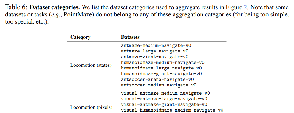
… a bunch of rows …
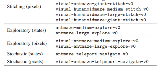
There’s only one dataset in each of the stochastic categories! I’m not sure what the reasoning here is. They say in the caption above that some are left out for being “too simple, too special, etc”. But it seems a bit weird to choose the only one that CRL is actually better on for the stochastic (states) category! Even if we look at the visual stochastic datasets (which there are only three of), it’s at least objectively the best… but for one of them (visual-antmaze-teleport-stitch-v0), it ties GCBC, and for another (visual-antmaze-teleport-explore-v0) it gets a score of 1, whereas HIQL gets 19, and all other methods get 0… so I’m not sure it makes much sense to say it’s the best there.
What’s going on with the max Q/V values?
In my training losses plots, I have it also plot some stats about the V and Q values in the batch. Here’s an example:

Something I noticed is that (squint, it may be hard to see here) the max values are above zero, and not just at the beginning of training, but until the very end. They’re not very much above zero, but they’re definitely bigger.
Why? Recall that in this GCRL setup, we’re using the sparse GCRL reward $r(s, g) = -\mathbb 1[s \neq g]$, i.e., it should be at most zero, and usually $-1$. The value functions should rack up this reward and be at most zero (hence the negative min and mean values you see for Q and V). I’m not generally surprised when VFs don’t match what they “should” be (and discounting makes it all even messier), but in this case they literally should never bootstrap off of a positive value. Further, GCIVL and GCIQL both use versions of double Q/V learning that make it choose the min target.
I can only think of two possibilities:
- There’s some part of the models that’s mapping some states to positive values, left over from initialization, and for some reason they haven’t been updated to be negative
- There’s some very weird generalization happening at states that are similar to legitimate $V \approx 0$ states (very handwavy, I know)
Still, strange. It’d be interesting to poke at this a bit more.
Offline RL… simple and stable? Did I suffer a head injury?
Mini soapbox rant :P skip to the next section if you don’t care.

At the top I mentioned I’m doing this partly because I want a “nice, simple, stable RL algorithm” to experiment with.
It might strike you as odd that I’m saying “simple” or “stable” about an offline RL algorithm, since they can be notoriously unstable, and to mitigate that, they’re often pretty complex compared to regular online RL algos. So I say that for two reasons:
First, IQL actually is pretty simple compared to most offline algos. It basically has typical RL models and doesn’t do anything too strange, or introduce some other crucial component that needs to be learned at the same time. Maybe it’s not the best, but it’s simple.
Second, despite the fact that offline algos are inherently unstable, they’re actually more reproducible in some sense, because they eliminate a huge source of uncertainty with online algos: rollouts and data collection. In your ol’ Sutton & Barto, the algos are usually shown with the training steps happening sequentially with your agent collecting data, usually doing a gradient step for each env step. In practice, it’s common to have many copies of the env running asynchronously, all inserting into a replay buffer that a trainer samples from, to increase sample production throughput. This makes sense, but it can really complicate things.
Orthogonal to the async aspect, even having to collect data from an env at all adds another step where crucial stuff is often snuck in. “Oh, we just clip the actions to range XYZ” or “we added a reward offset because our uncle said it’s good to” or “we decided to terminate the episode when the robot falls over or went to a location that isn’t as cool”. Sometimes people are clear about this stuff, sometimes it’s snuck into an appendix, sometimes it’s only in the published code, and sometimes there’s literally no way to know. And that’s not even getting to the fact that people might be using different versions of envs.
Anyway, rant over! My point here is that works with offline RL algos tend to dodge this trouble, since they’re usually learned from a static dataset you can go and download. There are still potentially some of the same problems when you go to evaluate your trained policy (see my IQL post), but it’s a lot simpler in that respect.
Minor differences from last time
It’s worth noting that the three algos I’m doing today aren’t inherently GC – you can basically turn any algo into a GC version of it by augmenting the state input of the models with a goal input $g$. For example, instead of $Q(s, a)$, now you have $Q(s, a, g)$ (OTOH, the other three algos really do have GC as a foundational part of them!). That said, there are a few important differences.
IVL
First, one of the algos is a version of IQL called IVL. In IQL, we had two state-action VFs, $Q_1, Q_2$ (to do double Q learning), and a target function $\bar Q_i$ for each of them, and then a single state VF, $V$. For a transition $(s, a, r, s’)$, the TD target for each $Q_i (s, a)$ is $r + \gamma V(s’)$, and for $V(s)$, it minimizes the $\tau$-expectile loss $L_2^\tau ([\min_i \bar Q_i (s, a)] - V(s))$. So the Q functions bootstrap off $V$, and $V$ tries to match the expectile over actions of the (target) Q functions.
In IVL, they do away with the Q functions entirely. To do this, they just replace the Q in the expectile loss with… what it was basically trying to approximate anyway! I.e., for transition $(s, a, r, s’)$, they replace $\bar Q_i (s, a) \mapsto r + \gamma V(s’)$ in the $L_2^\tau$ loss. However, you don’t want a function bootstrapping off itself, so they have a target state VF $\bar V$. And since they still want to mitigate overestimation bias, they actually have two state VFs $V_1, V_2$, and a target VF for each.
That still leaves a couple questions about how you might choose to do parts like the double VF learning and the expectile loss that they don’t mention in the paper, but luckily they’re very clean in the code with a couple tricks they’re using.
And of course, both the IQL and IVL are GC versions – so the models are $Q(s, a, g)$ and $V(s, g)$.
Policy extraction - DDPG + BC
IQL only learns value functions, so you still need to extract a policy from those. In the IQL paper, they use AWR to do this. However, in the same authors’ similarly impressive paper “Is Value Learning Really the Main Bottleneck in Offline RL?” (2024), they found that the policy extraction method is really important for getting a good policy in offline RL. They found that AWR actually isn’t a great choice, and a better one is what’s usually called “DDPG+BC”, from the similarly no-bs paper “A Minimalist Approach to Offline Reinforcement Learning” (2021).
It basically just takes your learned Q function, and does a DDPG style policy update by plugging the policy output $\pi(s)$ into $Q(s, \pi(s))$ and taking the gradient of that with respect to the policy parameters, with the tiny addition of adding a behavior cloning (hence the BC) term, giving the objective:
\[\mathbb E_{(s, a) \sim \mathcal D} \bigg[ Q(s, \pi(s)) + \alpha (\pi(s) - a)^2 \bigg]\]I.e., maximize $Q$ while not straying too far from the actions in the dataset. The tradeoff between those two competing terms is determined by the “temperature” parameter $\alpha$, similar to AWR (but inverted).
Since this would be tricky to do with just state VFs, they only use DDPG+BC for GCIQL, and still use AWR for GCIVL.
Goal sampling
The last detail is how the goals are actually sampled. A key concept in GCRL is “goal relabeling”, which briefly means relabeling trajectory data to say the goal was actually whatever you want it to be. The reason this is useful is that if you have a trajectory $[(s_1, a_1), (s_2, a_2), \dots, (s_N, a_N)]$, regardless of what the agent that produced that data was trying to do (and whether it succeeded or not), you can after the fact “relabel” the trajectory to say that the goal was actually $g = s_N$, in which case it was a successful trajectory! And then, use this to update your models.
In the OGBench dataset, it’s not like the trajectories are labeled with their “real” goals and this is a trick we can do by ignoring them – there actually are only trajectories of $(s_i, a_i)$ pairs! I.e., it’s like we were handed a big pile of raw data and we have no idea what the agent that produced it was trying to do.
So, when we want to update our models (which now take a goal input $g$, remember), we need to do this labeling to choose what the goal is for each transition. Concretely, we’re going to sample a transition $(s, a, s’) \sim \mathcal D$ the way we usually do for an update step, but we also need to produce a goal $g$. $g$ will be plugged into the models, but it’s also where all the learning signal actually comes from! The sparse GC reward function is $r(s, g) = -\mathbb 1[s \neq g]$, and the termination (“done”) $d(s, g) = \mathbb 1[s = g]$ depend on it.
This is a pretty important detail. For example, if we only randomly sampled $g$ from the whole state space, in a continuous space we’d never have $s = g$, and would always get $r = -1$ and never terminate an episode. Since every transition would receive the same exact information, the value functions wouldn’t learn anything!
So you need to sample goals from states in the dataset, so at least some transitions will have positive learning signals. However, on its own this wouldn’t be enough. For example, in the pic below with three trajectories, if we had the transition $(s_3, a_3, s_4)$ from trajectory $\tau_1$, and sampled a goal of $g = s_6$ from traj $\tau_3$, it’d still have $r = -1$ and not be super helpful:

To form a sample that actually gives reward/done, we need to sometimes choose the current state of the transition to be the goal, $g = s$, so if we sampled $(s_3, a_3, s_4)$, choose $g = s_3$ (giving $r = 0$ and $d = 1$).
However, doing only this wouldn’t be good by itself either – it’d only be training the models to know that it’s good to be at the goal, but not how to get to the goal.
Therefore, it’s also common to sample goals from future states of the same trajectory the transition came from. For example, if we sampled transition $(s_3, a_3, s_4)$ from traj $\tau_1$, we could sample $g = s_6$ from $\tau_1$. This would allow the value functions to back up the signal from the samples where we did use the $g = s$ goal. Sampling from the same trajectory is commonly done with either a uniform distribution or a geometric distribution over following states.
Lastly though, coming back to where we started, you probably do still want to choose random dataset states sometimes! I think this is to encourage generalization across trajectories, though I’m not 100% convinced of this. Here’s my thinking. Imagine we have these two trajectories, and at some point during both of them, they both encounter a state that’s very similar (but not identical) to a state in the other. In this case, state $s_4$ of both traj’s are similar to each other:

If the two states are similar enough, we’ll get some generalization in the value functions, where $V(s_4)$ will be similar to each other for the $s_4$ in both traj’s (which I’m showing with the dashed circles around each). If that’s the case, then if we had the transition $(s_2, a_2, s_3)$ from $\tau_1$, it could still get useful info if it sampled $g = s_6$ from $\tau_2$, which I’ve highlighted the effective path of with the red arrows.
However… I’m not totally convinced of this. Won’t it happen automatically?
Anyway, in practice, they do… all of them! They essentially form a hierarchical distribution, by first determining which goal sampling style they’ll do, by sampling a categorical (over “current state”, “future states, uniform”, “future states, geometric”, and “random dataset states”), and then sampling from the chosen distribution. They choose different weightings across these depending on both the policy vs VF goal, and the given dataset.
This part is pretty interesting to me, and I’d like to learn more about what makes it work and not work. From a kind of handwavy view, it actually seems like a key skill humans naturally have: we learn pretty well what states we can reasonably generalize across, and which ones we can’t, which is crucial for knowing if a plan is likely to work or not.
Donezo
Okay, that’s all for today! A lot of this was just getting stuff set up in a different way (in terms of my code), but the algos and datasets themselves were waaay simpler than last time.
Next time, I’ll be looking at some of the other methods, since I think they have some promising and cool aspects. Whereas the ones I’ve looked at so far have been pretty straightforward extensions of typical RL algos to be GC versions, the other ones they look at in this paper are weirder and not quite typical RL algos (CRL and QRL especially).