Touching grass: offline RL with the IQL algorithm

Today’s post is on a widely used offline RL algo called IQL, from “Offline Reinforcement Learning with Implicit Q-Learning” (2021). I implement and reproduce what I can of it, although… it’s a battle. I’ll write up what I got so far, and maybe come back to this later to fix what I can’t get here.

Oooh! Ahhh! Look at it align that pen.

Preliminaries

Off… line RL? and the situation at hand

I’ll assume you’re familiar with the distinction between on- and off-policy RL algos. The problem offline RL algos are trying to solve is kind of the extreme case of off-policy algos: you’re given a static pile of data from some environment, collected by god knows what means, and you want to get a policy out of it that would do well if you then deployed it into the real env.

For example, imagine we sent a robot on a mission to another planet (to make this story work, let’s assume that the robot can’t do any training on its own because it has very little RAM, and it also can’t receive signals because of crazy space stuff, but it can send signals 😉). So our robot collected and sent data back to earth for some period of time, before meeting its untimely demise.

Now we’re preparing our next mission to the same planet, and we’re training a new robot. All we have to train our new robot is the data that the old dead robot sent back.

So here’s the scenario we want to solve: we have a dataset $\mathcal D$ of a fixed number of trajectories from some env, where trajectory $j$ is $T^j = [(s_0^j, a_0^j, r_0^j), (s_1^j, a_1^j, r_1^j), \dots, (s_n^j, a_n^j, r_n^j)]$, basically what you’d expect. Then… we do whatever we want with that dataset, and want to produce a policy $\pi(a \mid s)$. We typically evaluate the final policy by actually running it in the environment and looking at its returns.

Note that we generally don’t know how the data was collected, so it might be from a lousy policy, or a mix of policies, and may be missing big parts of the state space, or actions taken in some states.

The simplest method (BC)

The simplest method we can use for an offline dataset is probably Behavior Cloning (BC). The idea here is to basically treat the problem as a supervised learning problem, where we train the policy to map states to actions: $\pi: \mathcal S \rightarrow \mathcal A$. Since generally there’ll be different actions taken in a given state, it’s more like a mapping from states to a distribution over actions, $\pi: \mathcal S \rightarrow \mathcal \Delta(A)$. This is usually done by parameterizing $\pi$ as a Gaussian, and then just maximizing the log prob of the actions in the dataset, so the objective is $J(\theta) = \mathbb E_{(s, a) \sim \mathcal D}[\log \pi(a \mid s)]$.

This can work well enough in some cases. If your dataset was collected by a very good agent, BC would produce a policy that just imitates the dataset, and it’d probably work well enough. But…

The problem with the simplest method

You might’ve noticed that the BC objective doesn’t use the rewards $r_i$ at all! Since that’s what we’d like our policy to maximize, it’s not surprising that BC is going to be pretty limited.

The most obvious way is that the BC objective basically causes the policy to match the dataset distribution over actions in each state. That means that even if the dataset actually contains all experience, good and bad, the BC policy will match the bad, along with the good.

For example, in this toy env:

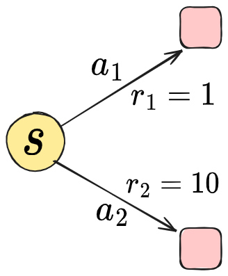
we have a single state, with two actions, each immediately ending the episode. $a_2$ is obviously the good action. If our dataset had a single sample of each action, so a 50/50 mix, the BC policy would also say to do $a_1$ half the time and $a_2$ the other half.

Booo! This clearly sucks. We have all the info! We should be able to get an optimal policy.

The problem with just using RL

Well, this is what RL algos are for. Why not use one of them?

There are a bunch of challenges, which is why offline RL is a whole research niche. But from a high level, most of it is the same trouble that off-policy algos have, but offline have worse. A major difference between them is that off-policy algos continue to collect data, so if your value functions (VF) have some delusion about the value of a given $(s, a)$ pair, eventually more data should be collected and updated with, and the mistake can ideally be fixed. OTOH, with offline, there’s no such feedback mechanism; the only data you have is what you were given!

More specifically and importantly for today’s post, a major cause of this is updating with out-of-distribution (OOD) actions. That is, if we look at the classic Q-learning update from a $(s, a, r, s’)$ tuple:

\[Q(s, a) \leftarrow r + \gamma \max_{a'} Q(s', a')\]

It’s bootstrapping off the Q value for the pair $(s’, a’)$. However, we might not actually have any data for that pair in the dataset! It only chose $a’$ because it maximized the Q value in that state. Therefore, if it’s incorrect about the value of $Q(s’, a’)$ because its value isn’t based on data, and we never get new data to correct it, this value will propagate back, potentially making the whole thing garbage.

So, we really want to avoid using OOD actions to update our VFs. There are a bunch of ways different methods use to do this, and IQL is one of them. But it’s a particularly simple idea. So let’s look at IQL!

IQL to the rescue?

Two phases: value learning and policy extraction

Many offline RL algos use an actor-critic setup, where the policy is being learned at the same time as the VFs, and both are used to update the other(s). IQL is a bit unlike most of them in that it learns the VFs first, and then a(n explicit) policy is extracted from them at the end. That is, the method is primarily about the VF learning, and agnostic to how the policy is extracted from those VFs. So, we can just focus on the VF learning here.

A simple way to never use OOD actions

There’s actually a simple way to learn VFs without ever bootstrapping off OOD actions. If we look at the SARSA Q function update:

\[Q(s, a) \leftarrow r + \gamma \mathbb E_{s' \sim P(s' \mid s, a), a' \sim \pi(a' \mid s)} [ Q(s', a')]\]

the expectation is over next possible states $s’$ (distributed according to the env transition dynamics) and next possible actions $a’$ in those states (sampled from the policy). Given a tuple $(s, a, r, s’)$, to approximate that expectation, you could sample $a’ \sim \pi(a’ \mid s’)$ to form it, but it’s also common to just use the next action from the actual trajectory that tuple came from. I.e., if the tuple was $(s_0^j, a_0^j, r_0^j, s_1^j)$ from $T^j = [(s_0^j, a_0^j, r_0^j), (s_1^j, a_1^j, r_1^j), \dots,]$, we can just use the action $a_1^j$ that followed state $s_1^j$, bootstrapping off $Q(s_1^j, a_1^j)$. That tuple is in the dataset, so we avoid sampling OOD!

…and why it won’t work

However, this will have a similar limitation to BC above. Any VF is always with respect to some policy, even if it’s implicit. In this case, the “policy” is implicitly defined by our dataset $\mathcal D$, so this algo will learn VFs for that policy. If we look at a slightly expanded version of the toy problem from before, where there are now just two consecutive action choices to be made in an episode:

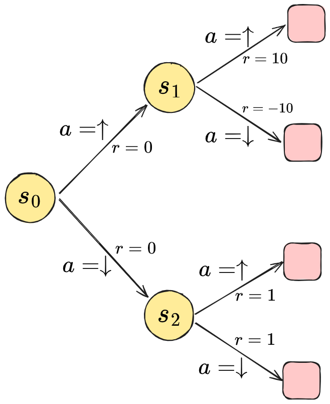
Assuming the env is deterministic, the best action sequence is $(\uparrow, \uparrow)$, giving a total reward of $10$. Let’s assume we’re lucky and we’ve been given a dataset that has total coverage, every action in every state! In each state, actions $\uparrow$ and $\downarrow$ were each taken half the time. What values will this learn using the SARSA method above? We’ll find that (assume $\gamma = 1$ for simplicity):

\[\begin{aligned} Q(s_1, \uparrow) &= 10 \\ Q(s_1, \downarrow) &= -10 \\ \Rightarrow \mathbb E_{a' \sim \pi(a' \mid s_1)} [ Q(s_1, a')] &= 0 \\ \Rightarrow Q(s_0, \uparrow) = 0 + \gamma\cdot 0 &= 0 \\ \\ Q(s_2, \uparrow) &= 1 \\ Q(s_2, \downarrow) &= 1 \\ \Rightarrow \mathbb E_{a' \sim \pi(a' \mid s_2)} [ Q(s_2, a')] &= 1 \\ \Rightarrow Q(s_0, \downarrow) = 0 + \gamma\cdot 1 &= 1 \\ \end{aligned}\]

So, despite having all the data we need, taking the greedy policy from the VFs learned using SARSA, it’d tell us that it’s better to go down in $s_0$! You can see why: the bootstrap for the next state is based on the dataset distribution over the actions, which is a lousy distribution compared to the optimal. Alternately, it’s saying that $s_1$ is a low value state, but it isn’t! It only looks like it is because bad actions are being taken from that state.

Finally, IQL

So this brings us to the clever ideas of IQL. We want to be able to make the bootstrap value $\mathbb E_{a’ \sim \pi(a \mid s’)} [ Q(s’, a’)]$ better than just based on the (potentially lousy) action distribution from $\pi(a’ \mid s’)$, but we also don’t want to sample OOD actions.

First, they bring in a state VF, $V(s)$, in addition to the state-action VFs $Q(s, a)$ we’ve already seen. The Q function loss is basically a typical squared error loss, but it bootstraps off $V(s’)$:

\[L_Q(\theta) = \mathbb E_{(s, a, r, s') \sim \mathcal D} [ (r + \gamma V_\psi(s') - Q_\theta(s, a))^2 ]\]

Nothing crazy here, but note that it’s only using real samples from the dataset for the bootstrap target. The neat part is in the loss for $V$:

\[L_V(\psi) = \mathbb E_{(s, a) \sim \mathcal D} [ L_2^\tau (Q_{\hat \theta}(s, a) - V_\psi(s)) ]\]

The magic is in $L_2^\tau$. Mathematically, $L_2^\tau (u) = \vert \tau - \mathbb 1(u < 0) \vert u^2$ (where $\mathbb 1$ is the indicator function), but I think a picture explains it a lot better:

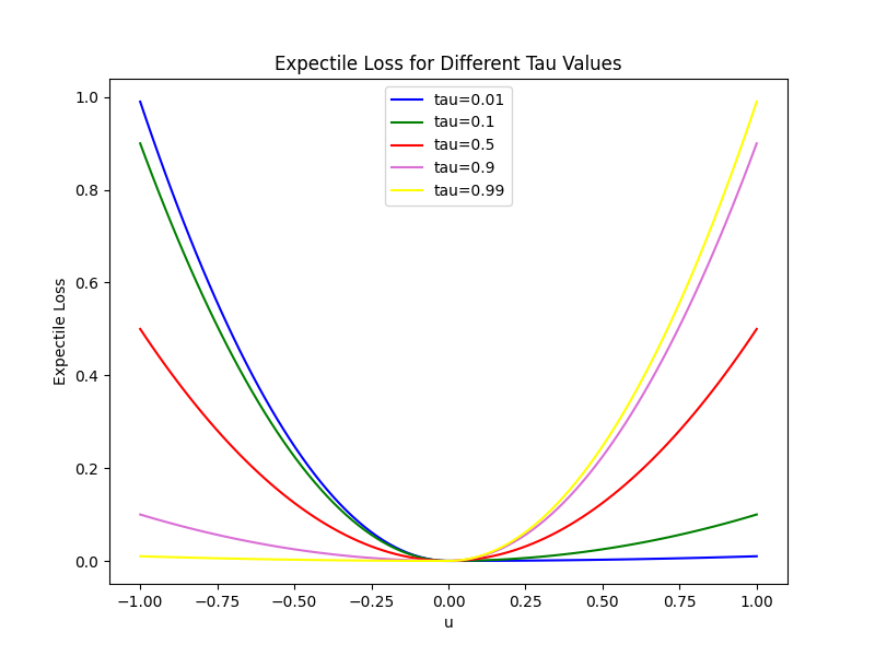
For $\tau = 0.5$, $L_2^\tau$ is exactly just a quadratic function, $0.5 u^2$ (red curve). But for $\tau \neq 0.5$, it weighs the $u^2$ part differently depending on whether $u$ is positive or negative. As $\tau \rightarrow 1$ (yellow curve), you can see that for $u > 0$, it’s basically the quadratic $u^2$, while for $u < 0$, it’s downweighted so heavily that it’s almost zero. Going back to how it’s used in IQL:

\[L_V(\psi) = \mathbb E_{(s, a) \sim \mathcal D} [ L_2^\tau (Q_{\hat \theta}(s, a) - V_\psi(s)) ]\]

You can see the effect this will have. The simple case of SARSA we looked at before corresponds to $\tau = 0.5$, because in that case, $V(s)$ is the mean of $Q(s, a)$, which minimizes $\mathbb E_{(s, a) \sim \mathcal D} [(Q_{\hat \theta}(s, a) - V_\psi(s))^2]$. But if we instead use a value $\tau > 0.5$ with $L_2^\tau$, $V(s)$ now tries to minimize that asymmetrically weighted quadratic, weighting positive errors more than negative ones.

If we go back to the two-step toy problem from above where we saw that with a 50/50 mix of actions in each state, SARSA would learn a lousy policy:

If we try it with IQL, $\tau > 0.5$, we find that:

\[\begin{aligned} Q(s_1, \uparrow) &= 10 \\ Q(s_1, \downarrow) &= -10 \\ \Rightarrow V(s_1) &= \arg\min_v \bigg[0.5 \cdot \tau (10 - v)^2 + 0.5 \cdot (1 - \tau) ((-10) - v)^2 \bigg] \\ &= \dots \\ \\ &= 10 (2\tau - 1) \\ \end{aligned}\]

$V(s_2)$ is the same as before, because $Q(s_2, \uparrow) = Q(s_2, \downarrow) = 1$ in both cases. So you can see that the bootstrap value of $V(s_1)$ is dependent on $\tau$ now. We can sanity check this by plugging in $\tau = 0.5$, giving $V(s_1) = 0$, like before. But now as we increase $\tau \rightarrow 1$, we see that the value IQL learns for $V(s_1)$ increases until it reaches… $10$! Which is unsurprisingly $\arg\max_{a, (s_1, a) \in \mathcal D} Q(s_1, a)$. So the value of $\tau$ basically lets us choose between SARSA and Q learning (more on that later).

The key thing here is that the distribution of actions is still the lousy 50/50 mix from before, but $\tau$ allows us to compensate for that. But, it’s not a silver bullet: if instead of that ratio, we instead had 10% $\uparrow$, 90% $\downarrow$, the problem would now be:

\[V(s_1) = \arg\min_v \bigg[0.1 \cdot \tau (10 - v)^2 + 0.9 \cdot (1 - \tau) ((-10) - v)^2 \bigg]\]

If you do the thankless arithmetic there, you’ll find that you need to use bigger values of $\tau$ than before to get the same value for $V(s_1)$; i.e., it has to compensate for the bad data distribution even more. Nevertheless, one of their key findings is that as $\tau \rightarrow 1$, it will approach the best VF that’s supported by the data (in theory).

Lastly, policy extraction

I’ll spend as little time on policy extraction as they do. Now assume that we’ve successfully got a $Q(s, a)$ and $V(s)$ that we trust reasonably, and we want to get a policy $\pi$ out of them. They use Advantage Weighted Regression (AWR), which is one of several similar variants. There’s nice theory behind it, but you can handwavily view it as BC, but where the log prob terms are weighted by a function of the VFs:

\[L_\pi(\phi) = \mathbb E_{(s, a) \sim \mathcal D}\bigg[\log \pi_\phi(a \mid s) \exp[\beta(Q_\theta(s, a) - V_\psi(s))] \bigg]\]

where $\beta \in [0, \infty)$ is an inverse temperature. You can see that $\beta = 0$ makes the exponential $1$, in which case it’s literally BC. For $\beta \rightarrow \infty$, the action with the largest Q value dominates and it effectively becomes an argmax over the actions at each state. Typical pattern: smaller temperature means “spikier” things, larger temperature means “smooshed” out, more averaging, etc. Again, note that it’s only updating $\pi$ with data $(s, a)$ pairs.

Enough talk! Let’s look at some experiments.

Experiments

Environments and datasets

They do a couple toy problems, but for the main results, experiment with four environments: mujoco locomotion envs, antmaze envs, Franka kitchen envs, and Adroit manipulation envs. Here are what a few of them look like:

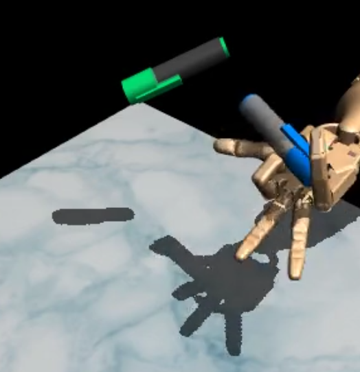
Each of those actually has a few different variants, with different state and action spaces.

For each env, they also look at the performance of algos trained on different datasets collected from those envs. Remember that above, we saw that “coverage” is the primary problem (i.e., handling the fact that the dataset might not contain all actions taken in all states), but also that the specific distribution of the data can be a problem too. So the different datasets provide different challenges to the algos. For example, here are the trajectory returns for the Mujoco walker2d “medium-replay” dataset:

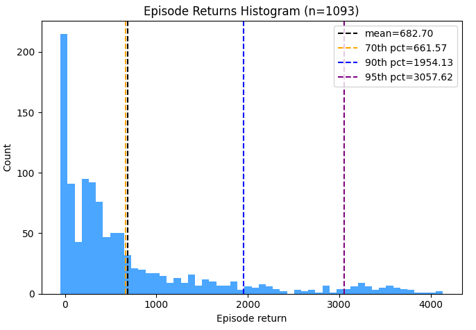while here are the returns for the walker2d “medium” dataset:

and here are the returns for the walker2d “medium-expert” dataset:

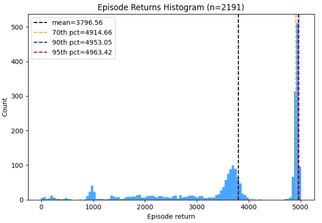You can see that the expert has “better” data, in the sense that it has that spike around ~5000. So it’s possible that training on the medium-replay or medium dataset could produce as good a policy as training on medium-expert, but it’ll probably be a harder task.

It’s worth saying that these envs aren’t crazy complex or anything, but they’re also not super simple either. Across the envs and variants in the paper, they have continuous state spaces of sizes ~10-60 and continuous action spaces of sizes ~3-30. Some of them also have tricky aspects like being a little “delicate” where one bad action breaks the episode.

I actually had a helluva time dealing with the envs and datasets, but more on that later.

Algos and comparisons

For each dataset, they test against “naive” baselines of BC, and a handful of previous offline RL/other methods: DT, AWAC, Onestep RL, TD3+BC, CQL. I’m not familiar with Onestep RL yet, and DT isn’t really an offline RL algo, but it’s a reasonable other comparison since it applies to the same problem setting.

For today’s post, I only implemented IQL itself and BC. Actually, they compared two versions of BC, regular BC, and “BC (10%)”. The latter is just BC, but you only keep the trajectories with the top 10% of returns, the idea being that if BC can be held back by having to place some probability on subpar actions, getting rid of those subpar actions from the dataset might help it. Anyway, I implemented that too since it was easy.

Some results

For the experiments, after training the VFs and extracting the policy, we run the policy in the corresponding env for some number of evals (I did $n = 300$). We then take a “score” for each eval (sometimes the return, sometimes something else; more on that nightmare later), take the mean of those scores across evals, and then normalize it by a reference score minimum and maximum (for that env), so the final number reported should be roughly in $[0, 100]$.

Their main comparison result is Table 1 in section 5.2, where they have a dataset per line and method per column, and break it into sections of the four main env groups (mujoco, antmaze, kitchen, adroit). Table 1 actually only has mujoco and antmaze, while the other two are in Table 3 in the appendix.

Here’s mine, for Mujoco:

\[\begin{array}{l||cccccc} \text{Dataset} & \text{BC (paper)} & \text{BC (mine)} & \text{BC 10 \% (paper)} & \text{BC 10\% (mine)} & \text{IQL (paper)} & \text{IQL (mine)} \\ \hline \hline \text{halfcheetah (medium)} & 42.6 & \textcolor{green}{42.4} & 42.6 & \textcolor{green}{42.9} & 47.4 & \textcolor{green}{46.6} \\ \text{hopper (medium)} & 52.9 & \textcolor{green}{46.6} & 52.9 & \textcolor{green}{47.4} & 66.3 & \textcolor{green}{54.2} \\ \text{walker2d (medium)} & 75.3 & \textcolor{green}{73.7} & 75.3 & \textcolor{green}{75.2} & 78.3 & \textcolor{green}{66.8} \\ \text{halfcheetah (medium-replay)} & 36.6 & \textcolor{green}{35.5} & 36.6 & \textcolor{green}{40.3} & 44.2 & \textcolor{green}{43.1} \\ \text{hopper (medium-replay)} & 18.1 & \textcolor{green}{11.6} & 18.1 & \textcolor{green}{63.8} & 94.7 & \textcolor{red}{29.0} \\ \text{walker2d (medium-replay)} & 26.0 & \textcolor{red}{11.8} & 26.0 & \textcolor{green}{47.6} & 73.9 & \textcolor{green}{62.6} \\ \text{halfcheetah (medium-expert)} & 55.2 & \textcolor{green}{48.5} & 55.2 & \textcolor{green}{88.9} & 86.7 & \textcolor{green}{81.1} \\ \text{hopper (medium-expert)} & 52.5 & \textcolor{green}{46.2} & 52.5 & \textcolor{green}{86.9} & 91.5 & \textcolor{green}{65.5} \\ \text{walker2d (medium-expert)} & 107.5 & \textcolor{green}{96.6} & 107.5 & \textcolor{green}{98.1} & 109.6 & \textcolor{green}{106.0} \\ \end{array}\]

For the three methods I did (BC, BC top 10%, IQL), I have the scores they got in one column, and then the scores I got for the same in the next column. I colored them green if they were at least 80% as good as theirs, yellow if 60% as good, and red if less than 60%.

You can see that for these datasets:

• I mostly got similar scores to them (more on that later)
• The BC methods got similar scores to IQL. Hmmmm.
• The BC 10% got as good, or sometimes much better, than plain BC

Here’s what I get for AntMaze:

\[\begin{array}{l||cc} \text{Dataset} & \text{IQL (paper)} & \text{IQL (mine)} \\ \hline \hline \text{AntMaze (umaze)} & 87.5 & \textcolor{green}{72.0} \\ \text{AntMaze (umaze-diverse)} & 62.2 & \textcolor{green}{48.7} \\ \text{AntMaze (medium-play)} & 71.2 & \textcolor{red}{11.7} \\ \text{AntMaze (medium-diverse)} & 70.0 & \textcolor{red}{5.0} \\ \text{AntMaze (large-play)} & 39.6 & \textcolor{red}{8.7} \\ \text{AntMaze (large-diverse)} & 47.5 & \textcolor{red}{4.0} \\ \end{array}\]

Ouch. Here’s Kitchen:

\[\begin{array}{l||cccc} \text{Dataset} & \text{BC (paper)} & \text{BC (mine)} & \text{IQL (paper)} & \text{IQL (mine)} \\ \hline \hline \text{Kitchen (complete)} & 65.0 & \textcolor{green}{59.5} & 62.5 & \textcolor{red}{2.2} \\ \text{Kitchen (partial)} & 38.0 & \textcolor{green}{55.5} & 46.3 & \textcolor{red}{25.8} \\ \text{Kitchen (mixed)} & 51.5 & \textcolor{green}{52.5} & 51.0 & \textcolor{red}{6.4} \\ \end{array}\]

and Adroit:

\[\begin{array}{l||cccc} \text{Dataset} & \text{BC (paper)} & \text{BC (mine)} & \text{IQL (paper)} & \text{IQL (mine)} \\ \hline \hline \text{Adroit Pen (human)} & 63.9 & \textcolor{green}{63.9} & 71.5 & \textcolor{green}{64.1} \\ \text{Adroit Hammer (human)} & 1.2 & \textcolor{green}{1.3} & 1.4 & \textcolor{green}{1.8} \\ \text{Adroit Door (human)} & 2.0 & \textcolor{green}{6.6} & 4.3 & \textcolor{green}{5.1} \\ \text{Adroit Relocate (human)} & 0.1 & \textcolor{red}{-0.1} & 0.1 & \textcolor{red}{-0.0} \\ \text{Adroit Pen (cloned)} & 37.0 & \textcolor{green}{56.4} & 37.3 & \textcolor{green}{63.1} \\ \text{Adroit Hammer (cloned)} & 0.6 & \textcolor{red}{0.3} & 2.1 & \textcolor{green}{2.8} \\ \text{Adroit Door (cloned)} & 0.0 & \textcolor{green}{0.4} & 1.6 & \textcolor{green}{2.1} \\ \text{Adroit Relocate (cloned)} & -0.3 & \textcolor{green}{0.0} & -0.2 & \textcolor{green}{-0.0} \\ \end{array}\]

Double ouch. My Adroit numbers are comparable, but really only because the paper also got really low scores for most of those envs. My Kitchen BC results are good, but that’s not really the point here (also note that their BC scores beat IQL!).

I’m a bit disappointed, since the Mujoco envs are expected to be kind of easy and Antmaze is supposed to be where IQL can really shine (since it has to do “stitching” of suboptimal trajectories), and that’s what mine had trouble with.

However… there’s a bunch to say about this. More on that in the discussion section below. For now, let’s gaze upon some videos produced by the offline policies above (with varying levels of cherry-picking depending on how successful it was for that env/dataset):

HalfCheetah:

Walker2d:

Hopper:

AntMaze Umaze:

Adroit pen:

Adroit door:

Wow! It sure opens that door, kind of.

Yadda yadda, afterthoughts, chin music

A little more discussion and intuition would’ve been nice

So, the expectile loss is really the star of the show in this paper, but the way it gets used with the Q and V value functions also seems pretty important, and I felt like they glossed over it. Another part that would’ve been nice to discuss a little more is the downside of larger $\tau$ values. They do mention:

Therefore, for a larger value of $\tau < 1$, we get a better approximation of the maximum. On the other hand, it also becomes a more challenging optimization problem. Thus, we treat $\tau$ as a hyperparameter.

It’s clear why larger $\tau$ approaches the maximum, but the more challenging optimization downside is less clear. I assume they mean: in the VF loss, $L_2^\tau (Q_{\hat \theta}(s, a) - V_\psi(s))$, larger $\tau$ means there will be fewer $(s, a)$ for which $Q(s, a)$ is large enough compared to $V(s)$ that the asymmetric loss won’t effectively ignore it. But I’m not confident about that for a few reasons. It would’ve been cool to see a figure similar to their Figure 3 (where they show that you need a larger $\tau$ for some of the AntMaze tasks to get good behavior), where they show the effect of going too high with $\tau$ and getting much slower learning.

Post training vs concurrent policy extraction?

This is another confusing aspect of my results. Like I mentioned above, the main value learning of IQL happens completely independently of the policy, so the policy can be extracted by any method afterwards.

But of course you can just extract the policy at the same time you’re learning the VFs, where it’ll be learning from not-fully-baked VFs (i.e., like what’s done in a typical AC algo). And that’s what they do in the paper:

Note that the policy does not influence the value function in any way, and therefore extraction could be performed either concurrently or after TD learning. Concurrent learning provides a way to use IQL with online finetuning …

They give one sort-of reason to do concurrent policy training, but I suspect another is just that you’re already sampling from the dataset and doing training, so it’s simple and probably overall faster to do that, than doing a whole separate training loop after (and aesthetically, I think people probably prefer an “all in one” training rather than awkward separate stages).

However, you might reasonably think that concurrent training is at best the same as post-training policy extraction, and plausibly worse. I.e., the VFs go from terrible at the beginning of training, to good by the end, so concurrent training is both trying to hit a moving target, and that target is also incorrect for much of the training. It’s possible that it might not matter too much (after all, most online RL algos are doing a more complicated version of this, i.e., “general policy iteration”) and the concurrently trained policy ends up also being good.

So I had my setup do both, train a policy concurrently, and then also train another policy after the fact with the final VFs. What was really surprising is that for most of the datasets, the after-the-fact policy was worse! For a few it was better, but usually worse.

I’m not sure what to make of this. It makes me wonder if I screwed something up, but it’s using all the same stuff for the post-train-extraction as for the concurrent policy learning, and also some envs get a better score for it. I’ll have to come back to it.

The envs and datasets are… a mess

Alright, so, this was probably the nastiest part of doing this whole thing.

In 2020, Prof. Sergey Levine et al published D4RL: Datasets for Deep Data-Driven Reinforcement Learning. Basically, offline RL was getting big, and there were problems with existing datasets and benchmarks people used, and of course there was the problem that it’s hard to compare different algos when everyone is using different datasets. Therefore, they chose a good spread of environments, and created some standard datasets that would be good tests for various challenges you might encounter in offline RL.

So a bunch of papers after that time were published using the D4RL datasets, including IQL. The trouble is that things move fast and code has a very short lifetime. A bunch of things changed:

• An organization called Farama took over the gym and other environments, since they weren’t being maintained
• If you go to the D4RL repo, you’ll see an announcement about that, and also that the D4RL datasets have now been “recreated” by Farama, as a project named Minari
• The envs that correspond to the D4RL datasets have also been upgraded several versions since moving to Farama; this is good because there were a bunch of bugs in the old ones

These all seem like improvements in terms of maintainability, documentation (much better with Farama!), and usage. However, there are also a bunch of difficulties I encountered.

Different env versions

First, the envs themselves have changed, i.e., the envs that produced the D4RL datasets and that the IQL results were evaluated on. So even when there is a Minari analog for a given D4RL dataset, like with the Ant Maze datasets, they’re now using very different env versions. For example, if you look at the version history for the Ant Maze envs in Minari, you can see that v1 and v2 are the legacy versions that were used in D4RL, but now they’re on v4 or v5, with some pretty big updates (more on that below). The newer versions are based on updated Mujoco bindings, and it seems like it’d be a pain to figure out which versions of several packages (gym, mujoco, tensorflow, d4rl, others?) I’d have to pin to get the old versions working.

I have no mouth and I must scream 😃

Some of the differences are minor, but at least a few of them are very significant. Primarily, AntMaze. Here’s an overview stats plot (that I have each run spit out) of the AntMaze Medium-Play dataset from Minari:

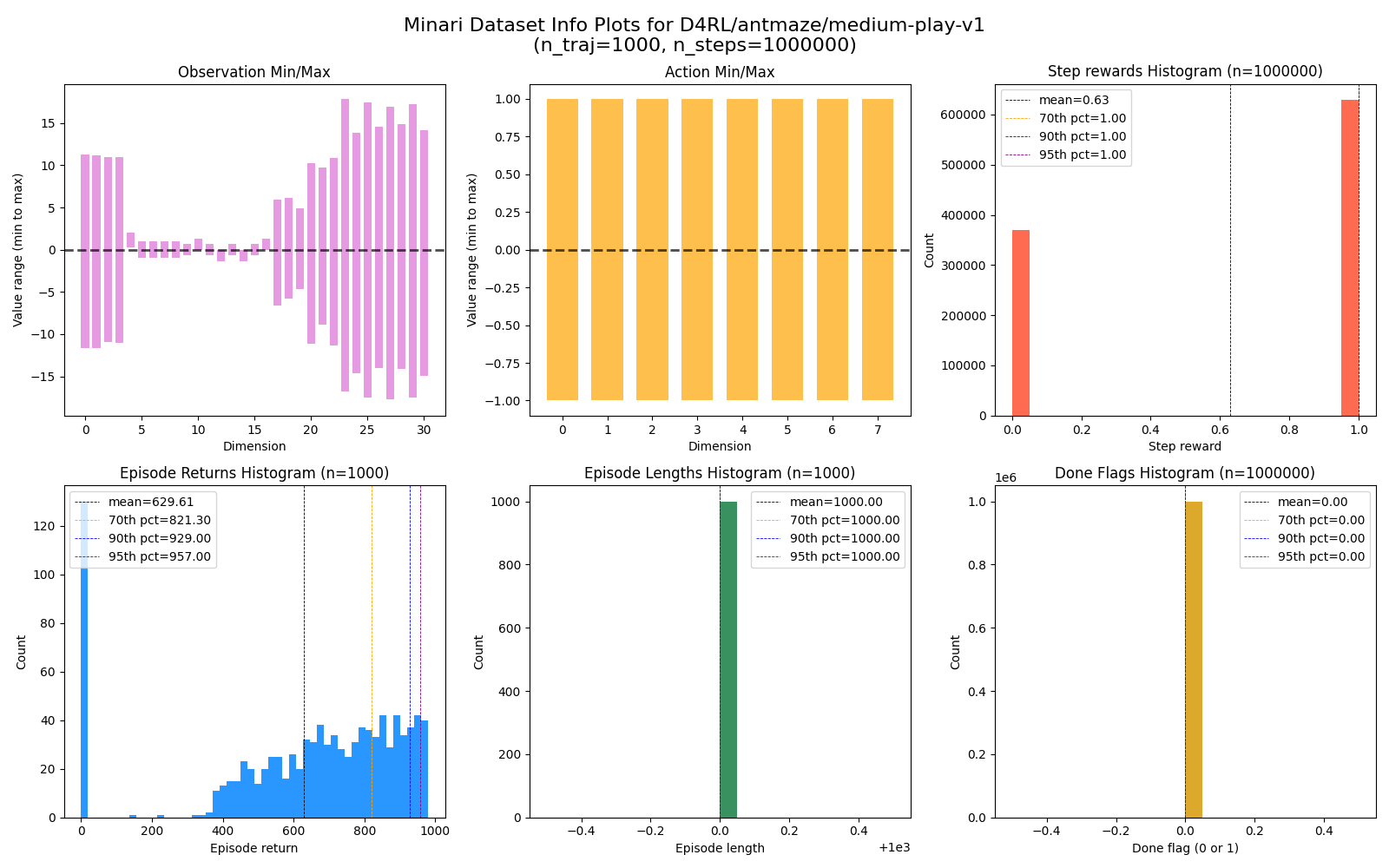
There are a couple things to highlight:

• The dataset is composed of 1k traj of 1M total steps
• All step rewards are 0 or 1 (red histogram)
• All episodes are length 1k (green histogram)
• Therefore, episode returns are between 0 and 1k (blue histogram)
• NO done signals (yellow histogram)

This reflects how the Minari AntMaze envs are set up by default: it’s a sparse reward where the agent gets $r = 0$ if it’s not at the goal, and $r = 1$ if it’s at the goal. If it reaches the goal, the episode does not end; it only ends after 1k episode steps, whether it ever reached the goal or not. So the done signal is always false, and if it reaches the goal before the 1k steps is over, it can just sit there and accumulate $r = 1$ per step.

In contrast, here’s the same figure but for the D4RL version I loaded:

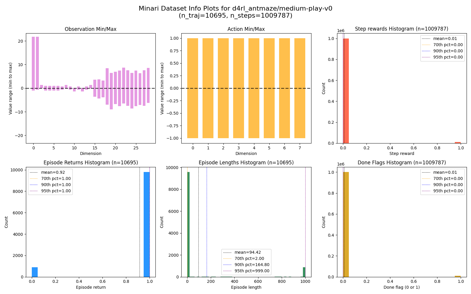
Here you can see:

• The dataset is a similar total size of ~1M steps, but has ~10k trajectories in it
• The episode returns are only ever 0 or 1 (blue)
• MANY episodes have a very short length (green)
• A nonzero minority of steps have $r = 1$ and done = True (red and yellow)

So despite being the same basic maze env, this older version has very different mechanics. It also has a sparse reward it only gets at the goal, but as soon as it reaches the goal, it gets a single reward of $r = 1$ and the episode ends with a True done signal. That’s why the returns are a maximum of 1, and why the vast majority of episodes have a length smaller than the maximum.

Alright, but why should it be easier with this version? I think the main reason is the number of trajectories: despite being the same total number of steps, the old D4RL version fits many more trajectories in those ~1M steps. In the Minari dataset, if the agent reached the goal in a given traj, that’s informative and useful for learning, but the following steps where it sits at the goal and just accumulates reward isn’t really useful at all (and look at the returns histogram! Some of those successful traj are sitting there for ~950 steps). In the D4RL one, those are replaced with steps from a different traj, which is probably more helpful for learning.

Related to this, I think there’s honestly just a bug in the old env. They mention something here in the version history that they fixed in v4 (version I’m using) that I think might be the cause:

Maze bug fix: Ant can no longer reset within the goal radius 0.45 due to maze_size_scaling factor missing in MazeEnv.

You might look at the D4RL episode lengths histogram above and think that the D4RL dataset just has a bunch of episodes where the agent starts extremely close to the goal (that first huge bin), but when I plotted a few trajectories in the dataset, I saw many many examples of…

I.e., two steps total. So my current guess is that 1) it had a bug where it’d often place both the agent and goal very close to each other, 2) it’d immediately end the episode with a positive signal, and 3) this makes learning a lot easier. It seems like even though those short episodes don’t give much helpful experience in terms of getting to the goal, they’re very helpful for learning what to do with the goal in all the different possible positions.

D4RL to Minari translation

Second, although they intended to recreate the D4RL datasets in Minari, there aren’t clear cut analogs for all of the old D4RL datasets in the IQL paper. For example, for the Mujoco envs in the paper, each env has the datasets “medium”, “medium-replay”, and “medium-expert”, while if you go to the corresponding Minari page, they now just have “simple”, “medium”, “expert”.

I think the hyphenated ones are datasets that are mixes of other ones, so you get some medium and some expert trajectories in the same dataset.

Minari version weirdnesses

Third, even within Minari, there’s some confusing stuff going on. For example, taking the Ant Maze Medium-Play dataset (a Minari analog of one of the D4RL ones in the paper), it’s a goal-conditioned env:

At the beginning of each episode random locations for the goal and agent’s reset are selected.

This is in contrast to an Ant Maze env like Umaze, which has a fixed goal and agent reset position for all episodes, which is obviously a lot easier to learn.

However, here’s the confusing part. If you scroll down to evaluation environment specs for Medium-Play, sometimes envs have an “eval env” where they restrict it somehow, and this one seems like it might, partly because other envs that don’t have a special eval env say so in their eval env specs section. Confusingly though, the actual specs you see for Medium-Play’s eval env appear to be exactly the same as the non-eval env…?

Unless… you happen to change the documentation version to a slightly less recent version. Current is v0.5.3. If you look at the same section for v0.5.1, you’ll see that the maze_map in the spec kwargs now reads:

{'maze_map': [[1, 1, 1, 1, 1, 1, 1, 1], [1, 'r', 0, 1, 1, 0, 0, 1], [1, 0, 0, 1, 0, 0, 0, 1], [1, 1, 0, 0, 0, 1, 1, 1], [1, 0, 0, 1, 0, 0, 0, 1], [1, 0, 1, 0, 0, 1, 0, 1], [1, 0, 0, 0, 1, 0, 'g', 1], [1, 1, 1, 1, 1, 1, 1, 1]], 'reward_type': 'sparse', 'continuing_task': True, 'reset_target': False}

I.e., you see a 'r' and 'g' where before there were 0. This is important, because the maze_map actually defines how the env is built and set up! 1 just means wall, but 0 means “agent or goal can be placed in this cell”, unless 'r' or 'g' are present, in which case those specify the static reset or goal positions.

The scores

Lastly, the scores. In the results tables above and in the paper, the numbers reported are “scores”. I guess they do this because different envs have different reward/return scales, and they want to be able to compare across them.

So what they do is take a “reference min” and “reference max” for each env, and then you take the mean results of your evals and scale it affinely so ref_min maps to 0 and ref_max maps to 100.

That’s mostly fine. But on top of troubles above, it adds another layer of “are my results in line with their results or not?”, because those normalization constants may have changed too. There are also some other complications. For example, the ref min and max for the D4RL/kitchen/* envs are (0, 4), but the returns are in the hundreds. Huh? It turns out that those ones are goal conditioned envs, with four goals, and the score is based on how many of those goals were achieved each episode, not the return (though goals achieved certainly leads to higher return). And, there’s something similar with antmaze envs that have goals. So there were just lots of little nasty surprises and remaining confusion there.

There are a bunch of hyperparameters and strange choices

I should be clear up front, in terms of RL algos, this isn’t actually too bad. But there are still a lot of seemingly arbitrary footguns and crucial parameters.

The most important are $\tau$ and $\beta$; the $\tau$ value will basically depend on the optimality of your dataset, and how much you want to deal with the “optimization challenge” they mentioned above. The choice of $\beta$ is a little more confusing; from a handwavy sense, I guess it should be based on how much you trust the learned VFs, so you can use a larger $\beta$ if you think it’s safe and you want the policy to ruthlessly exploit a slightly better action?

One worrying thing is the range of $\beta$ used across the envs; they use values of {0.5, 3, 10}, which is a factor of 20x between the biggest and smallest. The thing is, I think the $\beta$ value should interact pretty strongly with the reward/return scales, since where it comes into play is in the policy extraction, $\exp[\beta(Q_\theta(s, a) - V_\psi(s))$. So if you imagine scaling up all the rewards by some factor, that $Q(s, a) - V(s)$ advantage can now increase in magnitude too. So I think it would’ve been nice to normalize the dataset rewards for all the datasets in some way that makes them comparable, and then see what range of $\beta$ values are needed then. If it’s still a range like 20x, that’s not so good.

But there are other quirks:

• They standardize the Mujoco rewards by dividing the step rewards by the range of returns in the dataset. Okay, fine. But then they also multiply them by 1000! And don’t mention that part in the paper ☹️
  • dataset.rewards /= compute_returns(trajs[-1]) - compute_returns(trajs[0])
  • dataset.rewards *= 1000.0
• For the AntMaze envs, they mention that they subtract 1 from all the step rewards. This is common enough for “end the episode ASAP” tasks, but it’s still a little abnormal. They say in the code that it made no difference. I actually have some thoughts about what this reward structure difference might do with IQL, but I’ll leave that for a future post.
• For the Gaussian policies, they use a learned but state independent standard deviation. I.e., if your action space is 6-dimensional, they learn a vector of 6 log-standard deviations, and use that for all states
  • This is fairly unorthodox these days – I mean, you likely have much more data for some states than others, so it makes sense that you’d want your policy to have a much tighter distribution for the states where it’s very sure about the optimal actions.
• They apply dropout to the policy networks for the Kitchen and Adroit tasks to not overfit, since they have smaller datasets. Okay, whatever, just more complexity…
• They use a cosine LR scheduler for the policy. Nothing crazy, but another thing that makes it less clean.

---

Thaaaaaaat’s quite enough for today. I’ll definitely have a follow up IQL post where I try and figure out a few toy problem ideas I had, and also try and patch up some of the lousy behavior I found. Til next time!