Unrolling the Swiss - Isomap

Isomap, from “A Global Geometric Framework for Nonlinear Dimensionality Reduction” (2000), is one of about 80 trillion dimensionality reduction techniques that have been invented. I’ve been brushing up on a few of them, and Isomap follows very quickly from MDS, which I recently did a post on, so here we are.

The big picture

What’s the difference between MDS and Isomap? As I showed in the post on MDS, it produced reasonable enough 2D embeddings for some sets of 3D points, like this one:

but for others, it didn’t do so well:

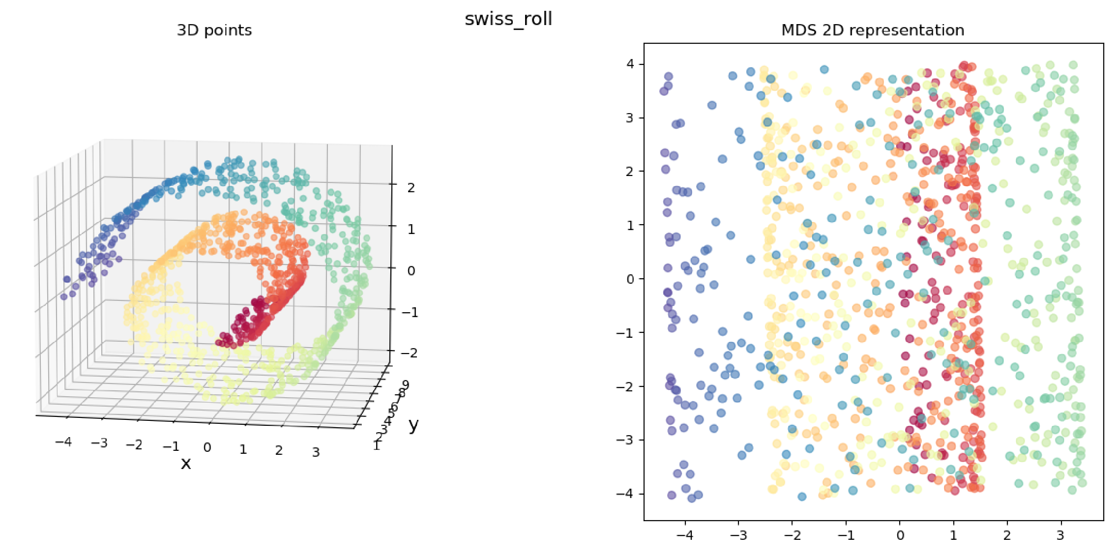
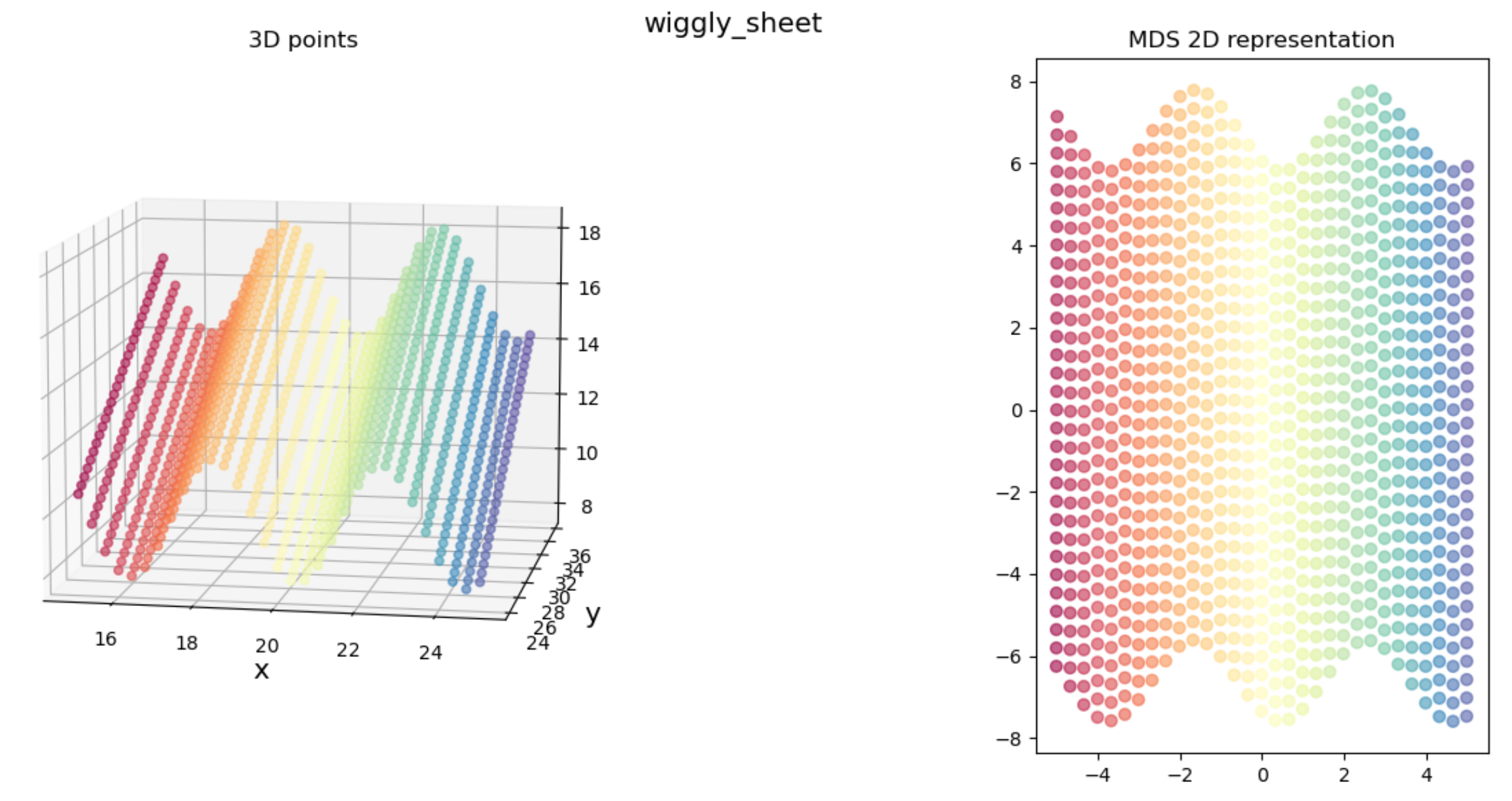
We clearly get the sense that in both cases, the true 3D shape is basically a 2D “sheet” that’s been deformed (being “corrugated” in the “wiggly sheet” example, and being rolled up in the “Swiss roll” example), so we’d hope that it’d find a 2D representation that reflects that for both.

This is what Isomap tries to do. It does an extra step that makes it so we can “unroll” the Swiss roll like so:

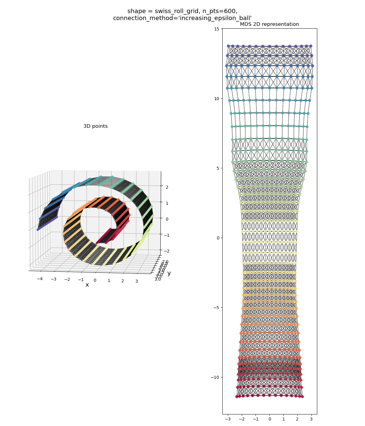
Isn’t that pretty! We’ve un-Swissed the roll. Or… unrolled the Swiss? I dunno, these are the type of questions that are above my pay grade.

How does Isomap work?

How does it work? Well, if you get MDS, you already understand about 90% of Isomap. If you don’t, check out my post on MDS first 😉

As a one sentence refresher: MDS assumes we have a set of $n$ objects and the pairwise distances between all of them, you choose a dimension $m$ that you want to embed these objects into, and then MDS tries to find coordinates (of dimension $m$) for each object such that the distances between each pair of objects in this new space is close to the distances we provided for them. Phew!

Importantly, MDS only cares about the pairwise distances between the objects; even if the objects are actually points in a higher dimensional space $\mathbb R^k$ (with $k > m$) than the space $\mathbb R^m$ MDS will embed them into, MDS doesn’t know or care. It just says “yeah yeah, just gimme the distances.”

On the other hand, Isomap does require points in $\mathbb R^k$. It takes a set of points, converts them into a specific distance matrix, and then just applies MDS to that distance matrix. And… that’s it!

The magic is of course in that “specific distance matrix” I snuck in there, but it’s actually pretty straightforward. Let’s motivate it with the example that MDS “failed” at above:

Recall that when we applied MDS to this, I literally just took those 3D points, calculated the Euclidean distance between each pair in $\mathbb R^3$, and then applied MDS to that distance matrix.

The problem with this is that if we look at the three points $A, B, C$ below, and the “naive” distances between them we’d calculate with MDS:

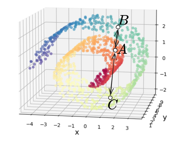
we can see that $d(A, B) < d(A, C)$. This is obviously true if we’re just considering them as unstructured points in $\mathbb R^3$ with no relation to each other. However, if we’re assuming that the Swiss roll is “actually” 2D, then you can see the trouble – the distances between those points should be more like this:

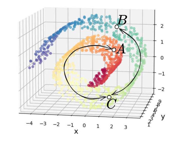
where now we have $d(A, B) \approx d(A, C) + d(C, B)$, which is then obviously bigger than $d(A, C)$, as we’d like.

Why does this happen? It comes down to the fact that in the 1st/naive distance case, we consider all of the points directly connected to all other points, while in the 2nd case, we’d like it so if you’re at point $A$, you have to “go through” point $C$ to get to point $B$, i.e., $A$ doesn’t “directly” connect to $B$ in the naive way.

This is what Isomap tries to do! The idea is to first create connections between each point and its neighbors such that all the points form a connected graph. Each point can use the local Euclidean distance as the distance to its neighbors (I’ve drawn some representative points as the circles below, as if the Swiss roll were much sparser):

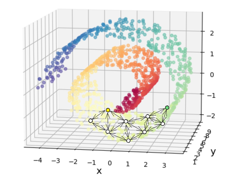
However, this means we’ll only have the distances between all points and their immediate neighbors, but since we do still want to MDS, we need the distances between each point and all other points. To do this, we just use a shortest path algorithm to calculate the shortest path between every pair of points, using only these connections/distances.

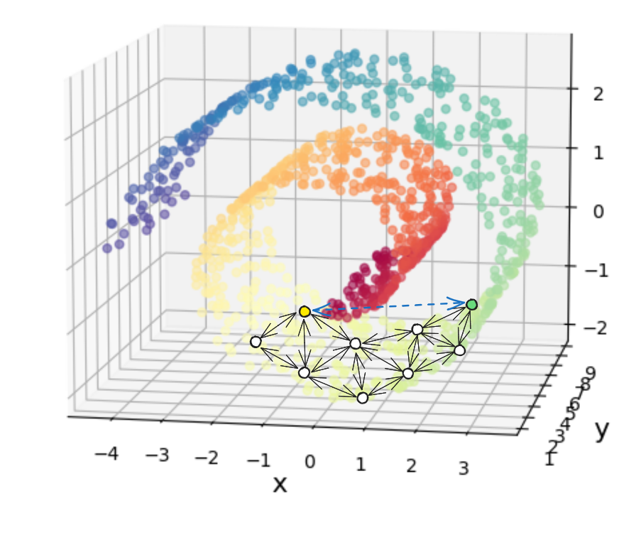
Now, if we look at the shortest path between the yellow and green points I highlighted, it would NOT be this dashed blue line (which is what the naive distance calculation would give):

and would instead be the sum of the highlighted blue connections:

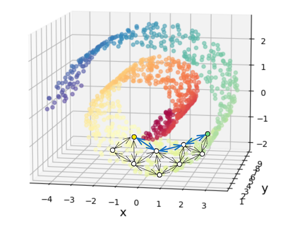
which you can see is longer, because it’s constrained to go along the Swiss roll.

After doing the shortest path algo, we’ll have the distance matrix between all pairs of points in the specific (😉) way we’d like, and we can naively apply MDS to it!

To summarize, Isomap is basically these steps:

• calculate the Euclidean distance from each point to its immediate neighbors
• use the Floyd-Warshall algo/etc to get the shortest path between all pairs of points
• apply MDS to those distances

That’s it! You can see that Isomap really isn’t adding a lot more, if you already get MDS.

Of course, the devil’s always in the details. Let’s give it a whirl!

A few results

Like I mentioned above, you can embed the objects into any dimension you want. However, it’s common to embed into $\mathbb R^2$ because it’s easy for us to visualize, and it’s also common to apply it to toy problems where the points are in $\mathbb R^3$, but are fundamentally a 2D manifold, so we can see if the process is working well (of course, going from 3D to 2D isn’t very interesting, and in practice we’d want to apply this to really high dimensional inputs).

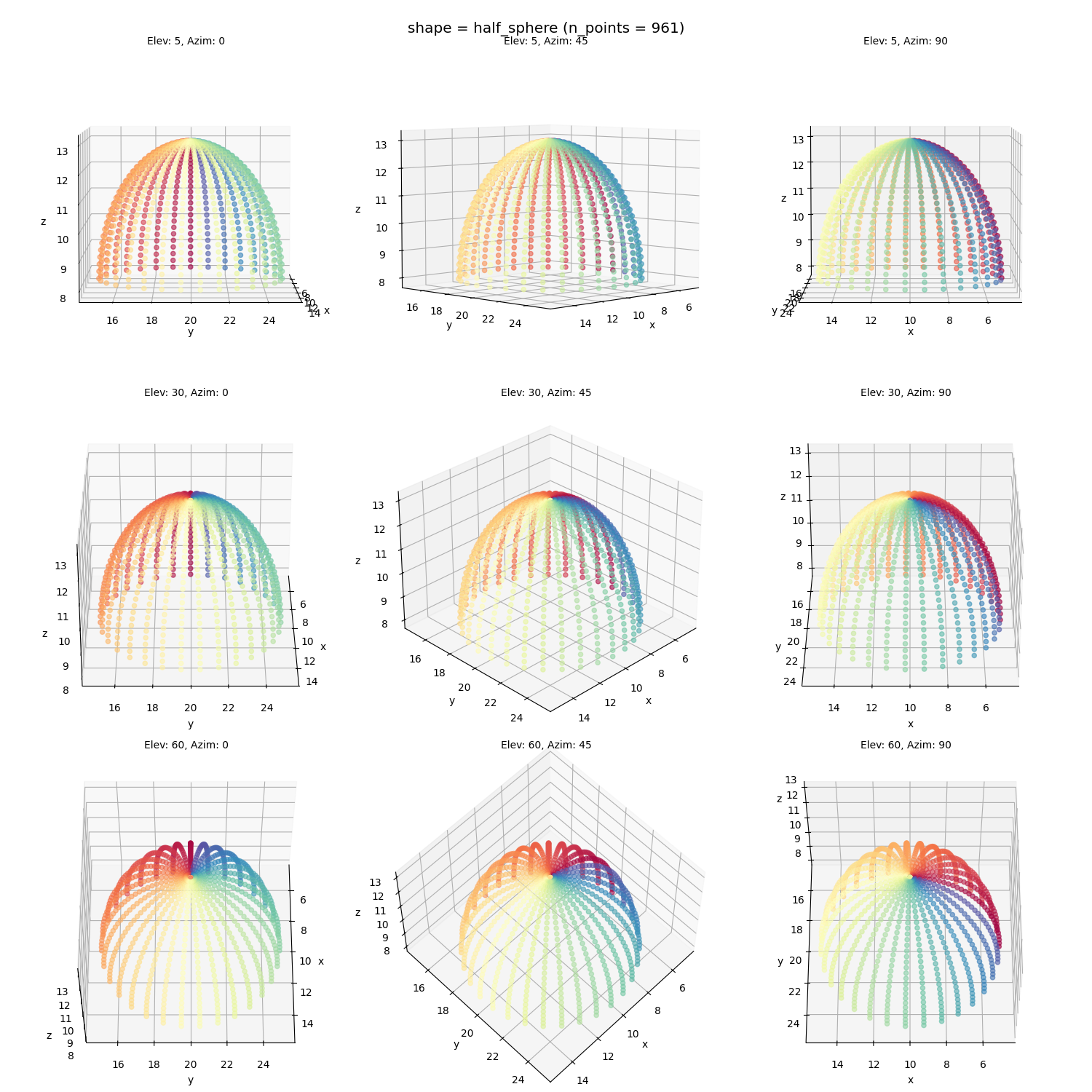
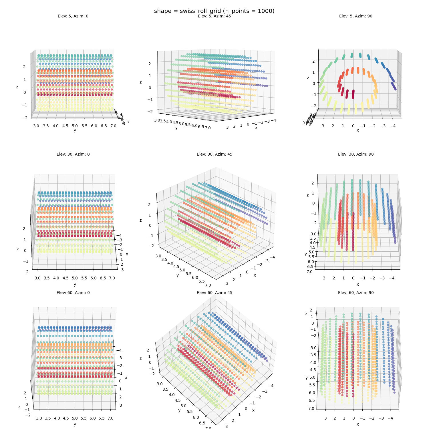
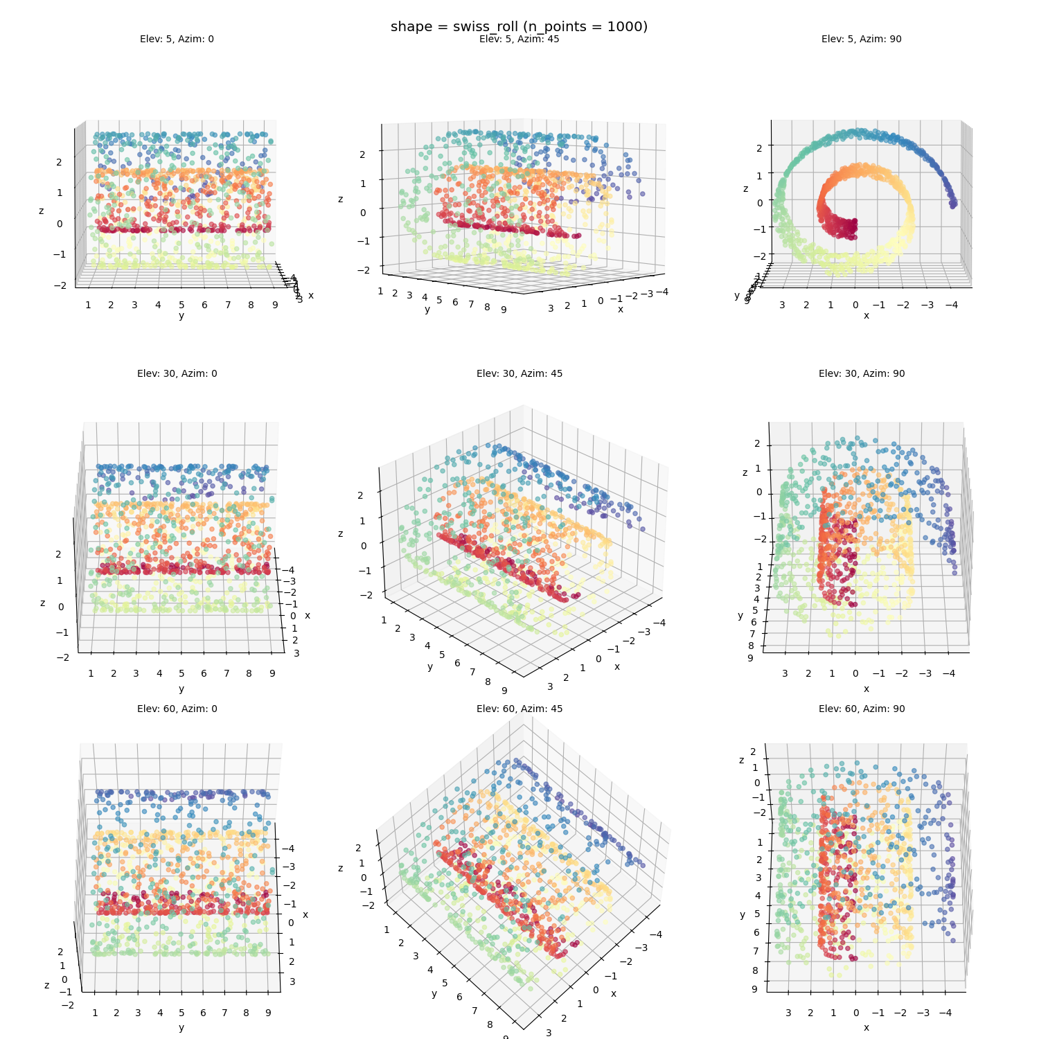
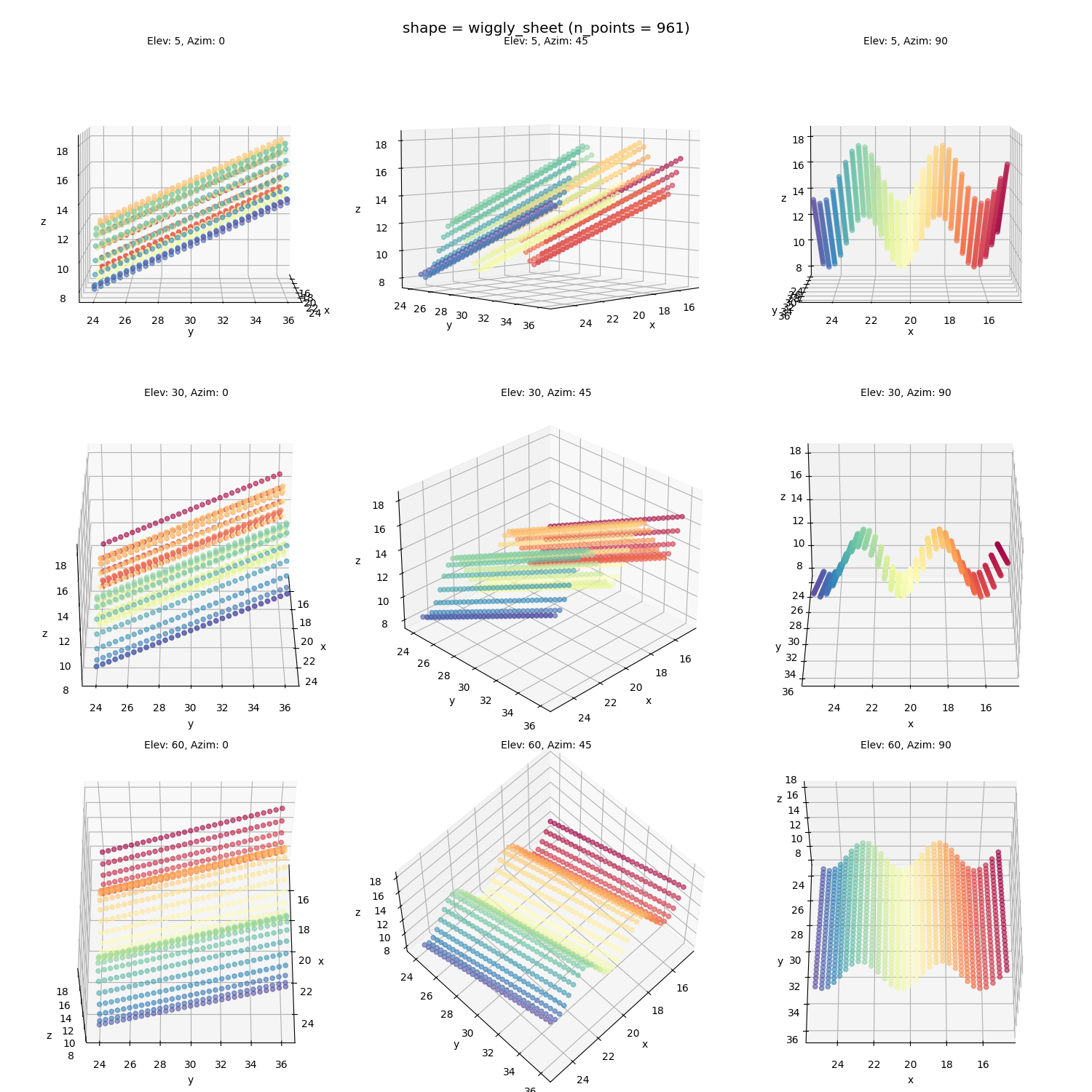
I chose a few 2D manifolds to apply Isomap to, to illustrate some challenges that some shapes have that others don’t. First I’ll show them with a variety of different views so you can get a sense of their shapes (which can be tricky with a single view in 3D). All of them are made of ~1000 points.

A half sphere:

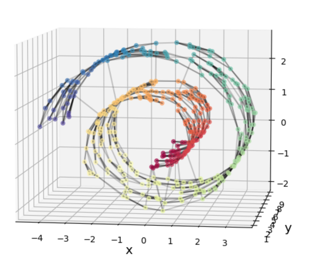
The Swiss roll with relatively evenly spaced points:

The Swiss roll with more randomly generated points (should be more challenging):

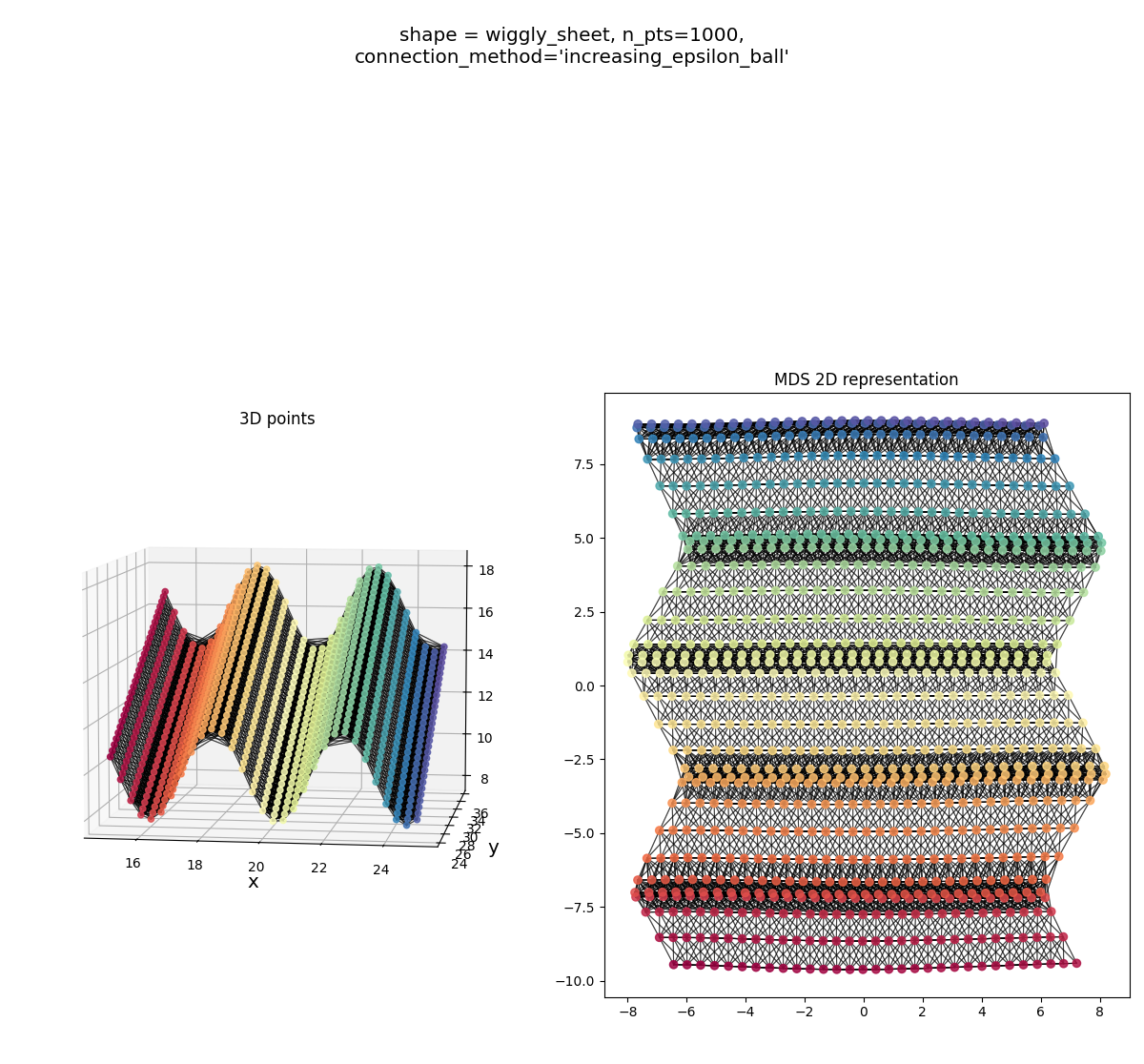
A wiggly sheet:

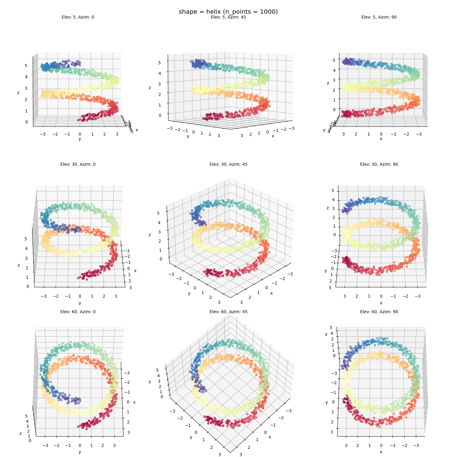
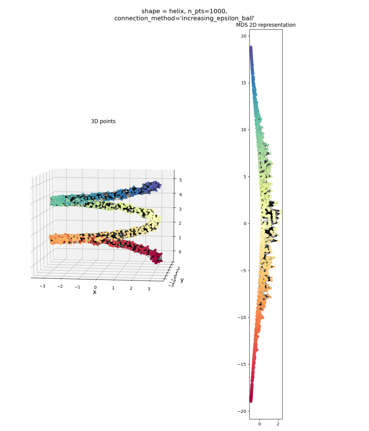
A helix:

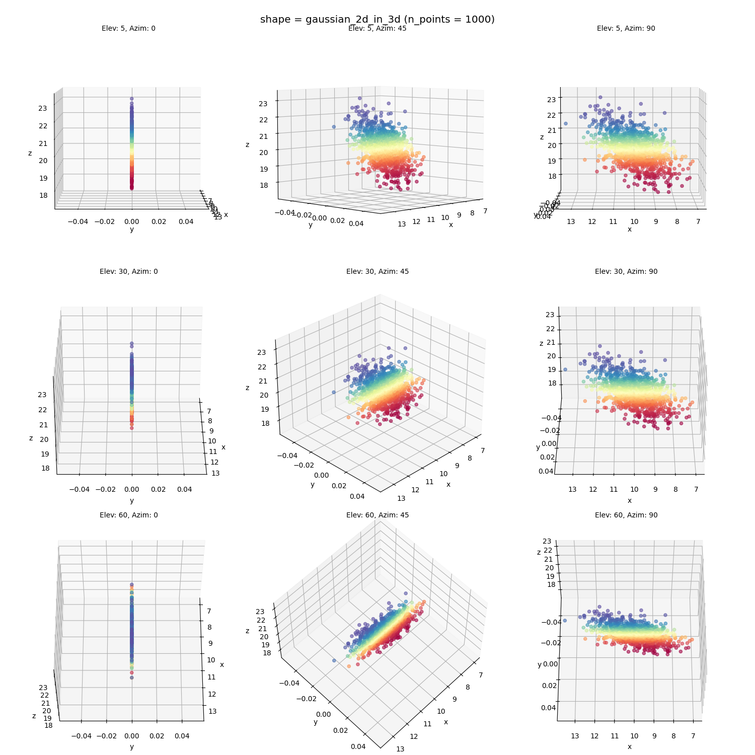
A 2D Gaussian, embedded into a slanted plane (this should be an easy sanity check, because it only occupies a 2D subspace in the 3D space already. Buuuut… see below):

Alright! Let’s look at how it does on them.

Half sphere:

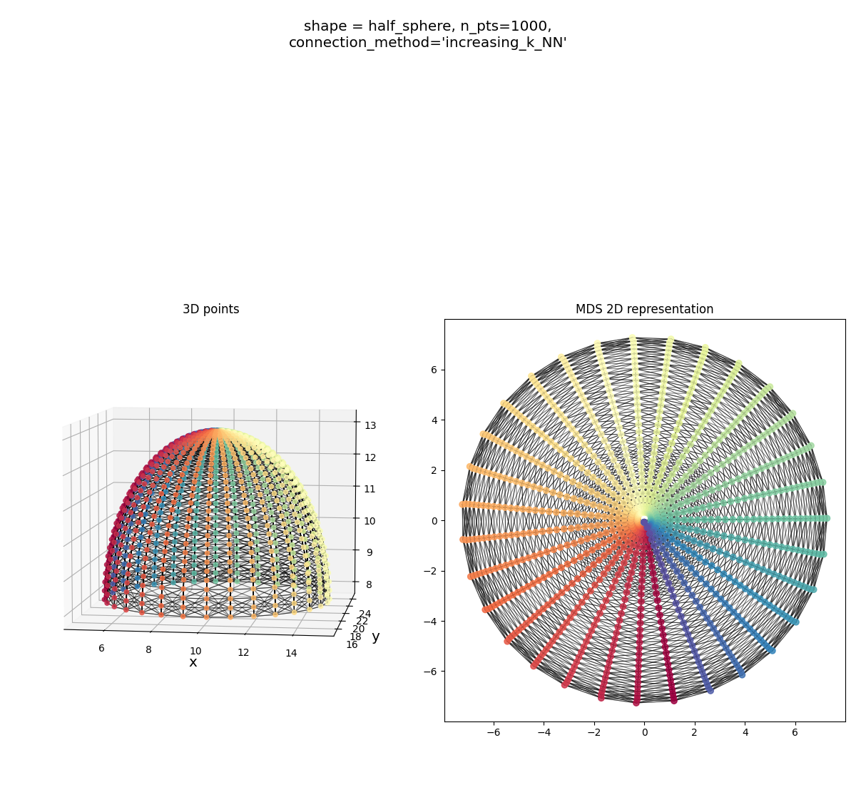
It gets the shape, but you can see a sign of trouble below:

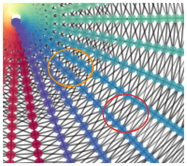
the connecting process has connected some points with a larger radius (circled in red) to their two neighbors the same radius, and the two at the immediate bigger and smaller radii, and the four at the closest diagonals. However, for some points at a smaller radius (orange circle), you can see that it’s connected it to a bunch of other diagonals too… This isn’t bad enough to mess up the shape MDS finds, but it’s not ideal. Additionally, there are probably connections that aren’t apparent here, where it’s connecting to several neighbors at the same angle.

Alternatively, if you use the $\epsilon$-ball, it’s really bad for this one:

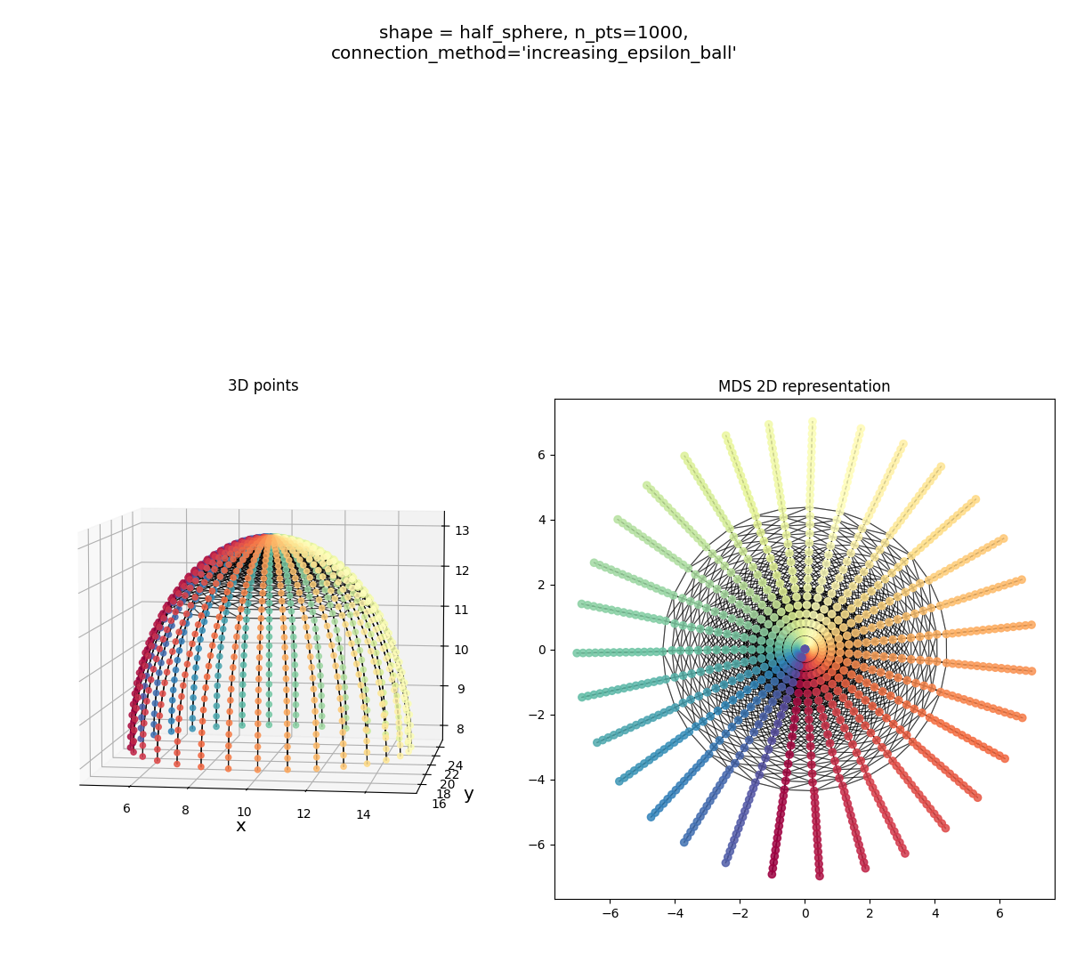
You can see that it’s able to fully connect the points with a pretty small $\epsilon$ value, but this has the effect of not connecting obvious “neighbors”… More on this in the next section.

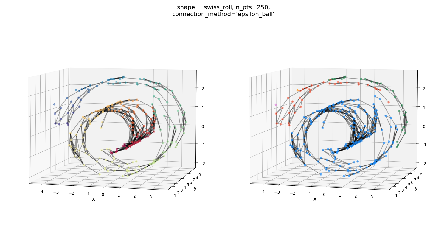
Swiss roll grid, both connection methods:

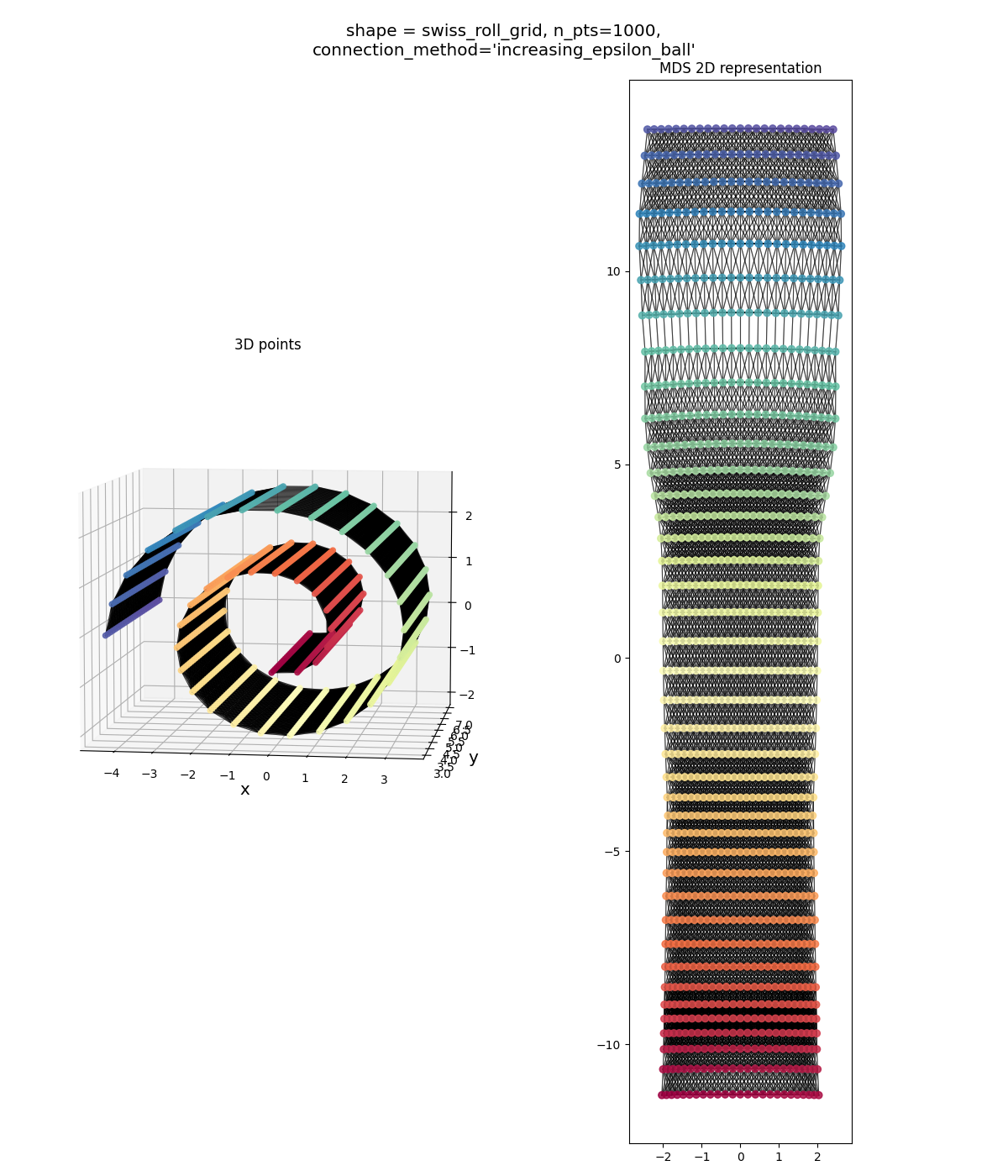
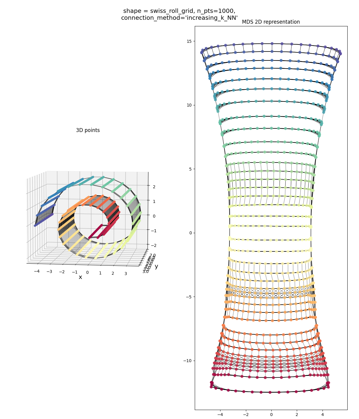
Similar story as above: one method seems to over-connect, the other seems to under-connect. Both aren’t bad overall, but over-connecting seems to be slightly better.

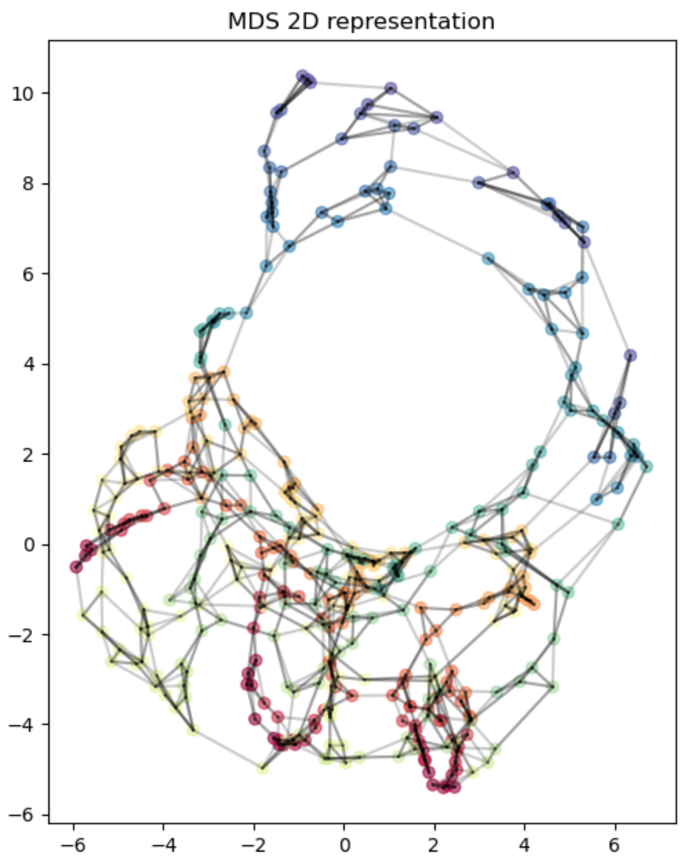
Swiss roll, noisy:

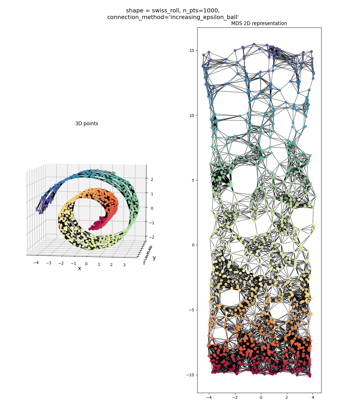
it’s obviously messier than a grid, but you know, that’s not bad! It’s definitely a high aspect ratio sheet.

Wiggly sheet:

Helix:

Finally, the genuinely 2D Gaussian on a tilted plane, which should be our “sanity check”:

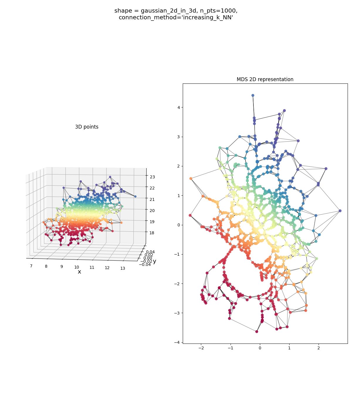
looks alright… could be better (the original points in red-orange definitely don’t have that huge hole in them that’s in the MDS points), but mostly there. But the $\epsilon$-ball version does:

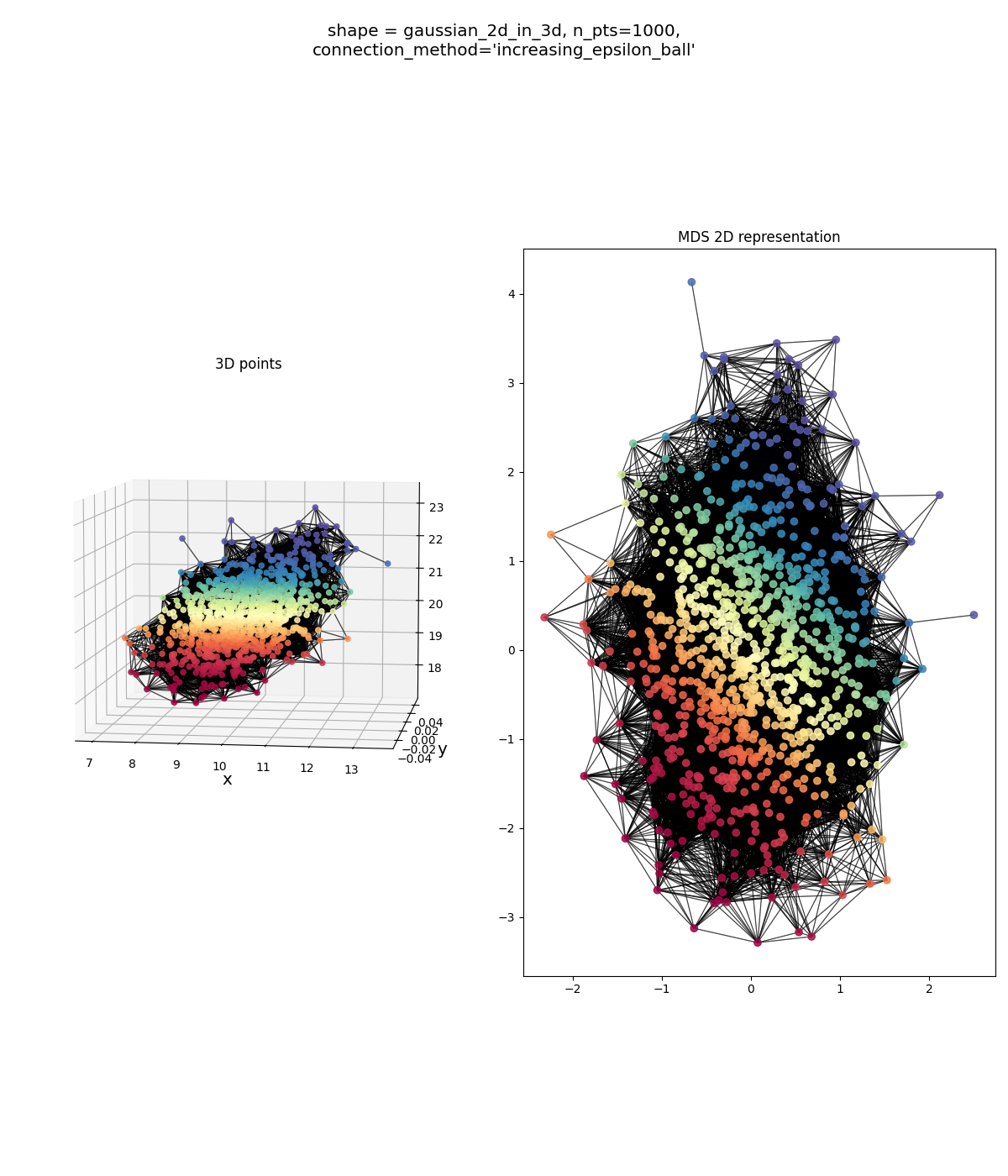
This is waaaaaaaay over-connected. You can see what’s likely happening: there are a couple blue points that are outliers in the original data. When we run the $\epsilon$-ball connection method, off the bat, the initial $\epsilon$ values probably connect the majority of points to their genuine neighbors, since they’re all pretty close and dense. However, those outliers will remain disconnected, so we keep increasing $\epsilon$ (only by 2% an iteration!) until we have a connected graph. By the time those outliers get connected, $\epsilon$ is way too big for most points, and most points have been connected to points that definitely aren’t their immediate neighbors.

And yet… qualitatively, I’d say the resulting MDS embedding actually has a shape that’s closer to the original data than the KNN yielded! I think the reason is that because the original data is contained in an actual 2D subspace (not just “inherently” 2D like the other shapes), adding these extra connections that the MDS will have to try and match the distance of won’t actually be much extra burden. OTOH, if we go back to this example from above:

and imagine we over-connected the yellow and green points with the blue dashed line, you can see that now there’s going to be a conflict in the distances of the embedded points no matter what. If we “unroll” the Swiss roll like it should be, the true neighbor distances (black arrows) will be accurate, but it’ll make this overconnection distance too large, etc.

Discussion

How you connect the neighbors can matter a lot

In the “how does it work” part, I kind of glossed over the part where we connect points to their neighbors to form a connected graph, before running the shortest path algo. Recall that we need a connected graph (i.e., there’s some path connecting any two points), because otherwise, the shortest path algo won’t ever connect some points, and the distance between them will effectively be $\infty$, which’ll break MDS.

It’s easy enough to understand the idea, but it turns out that the details of how you do it can be a real PITA.

They suggest two methods: 1) $K$ nearest neighbors (KNN), and 2) an $\epsilon$-ball based method. KNN means you connect each point to its… $K$ nearest neighbors (in terms of Euclidean distance in the original space). The $\epsilon$-ball method connects a point to all other points within a radius of $\epsilon$.

The first issue is that either method may not give you a connected graph if the parameter ($K$ or $\epsilon$) value is too small. For example, if you do the $\epsilon$-ball method and use $\epsilon = 10^{-5}$ but the closest two points are a distance of $10^{-2}$ apart, no points will be connected. More commonly, many points will be connected to each other, but there will still be a few big disconnected “clusters”.

Therefore, we can’t use a parameter value that’s too small, but we also don’t know a priori which value is good for the specific problem at hand. So for both methods, I start with a too-low parameter value, connect the neighbors with that value, check if the graph is connected yet, and then increase the parameter value if not, and repeat the process until it’s connected.

This ensures that we’ll get a connected graph, but the fun’s not over! As you might expect, using too high of a parameter value is trouble too. In this case, it means adding unnecessary / “incorrect” connections. While adding a few incorrect ones like this:

may not seem like a big deal, if we run MDS on this…

…we see that it’s really lousy! Briefly, this is because the extra edge acts as a “shortcut” for the shortest path of many pairs of points that should be quite far away. This actually turned out to be more interesting than expected and there’s more to say on this front, so I’ll stop for now and maybe do a future post on it.

Super un-optimized

I really didn’t optimize this at all, and there are a lot of opportunities for it. The biggest hit is the shortest path algo, which if you’re doing a naive Floyd-Warshall algo like I am, has a complexity of $O(n^3)$, with $n$ points. They briefly mention in the paper that there are easy improvements on that, but given the dynamic programming nature of it, I doubt the floor will be too low. Off the top of my head, I’d think that maybe something like a k-d tree could help, because in the step where you’re testing if a candidate distance between two nodes is shorter via going through a new node, you definitely don’t need to check all other nodes, and can likely just check a much smaller subset.

They made Isomap sound a lot fancier than it is

In my experience, there are topics where before hearing about them, you have the impression that they’re pretty simple, and then they turn out to have a lot more going on with them than you expected. ICA turned out to be like this when I did a post on it; I assumed it was just some linear algebra trickery, but it ended up having some really interesting bits about using non-Gaussianity, measuring negentropy, etc.

But sometimes you see the opposite, where the topic is gussied up real fancy, and turns out to be conceptually really simple, which is what I found with Isomap. This is partly because they use some unnecessary words from more complex topics like differential geometry (e.g., “geodesic distance”), to talk about concepts that are actually really straightforward.

Another interesting tidbit is that in the same exact issue of Science that this paper was published in, they published “Nonlinear Dimensionality Reduction by Locally Linear Embedding” (known as LLE), which is basically solving the same problem. Since it’s on literally the next page after the Isomap paper ends, and they also use the Swiss roll example, I have to assume that it was intentional to have them next to each other, but I’m still curious about the history.

Is there a right way to pick a dimension for the MDS?

After connecting points to make a connected graph and then applying the shortest path algo, you still have to actually choose an embedding dimension for MDS. In my case, the problems were artificial toy problems where I knew exactly their inherent dimensions. But in general, if we want to, you know, actually use this method on real data (!?!), we wouldn’t know the “true” dimension, if there even is one.

So I’m wondering, is there a reliable, automatic way to do this? (I’m sure there is, I’m just idly speculating without looking anything up.)

My first thought is a dumb empirical thing, where we take the fully connected (i.e., post shortest path algo) distance matrix, and embed it in increasing dimension, and compare the error of the embedded pairwise distances to the “true” distance matrix. Maybe if we’re lucky, we see a sharp falloff at the number of dimensions it “inherently” is.

Maybe a slightly more intelligent version could be trying to measure the dimension of the “tangent plane” at a given point. Before running the shortest path algo, we have the neighbors distance matrix. If you imagine a point on a 2D manifold, in a higher dimensional space, if we did a PCA-like procedure, we’d find that there are two main principal directions, with tiny amounts of variation in the others (due to curvature, noise, etc). Maybe using a global average of this could give us a good measure.