Multidimensional scaling - MDS

Multidimensional scaling (MDS) is a pretty old technique. It’s often said to be for reducing the dimension of data, but I think that’s not necessarily always true. Some people say it’s just a data visualization tool, but I think that’s also selling it short a bit.

What does it do, high level?

Here’s the big picture: we have $n$ “objects”, and assume we have the (symmetric) distance between each pair of objects. So these distances are represented by an $n \times n$ matrix, $D$.

We’ll then pick a target dimension $m$ that we want to embed these objects into. The MDS procedure will then try to find coordinates in $\mathbb R^m$ for each of the original objects, such that the distance between any pair of objects in this new $m$ dimensional space is the same as the distance we said for that pair in our distance matrix. Often, it won’t be possible to do this perfectly, so it’ll choose coordinates that are the best compromise.

It’s pretty common for these “objects” to be points in some Euclidean $\mathbb R^k$ space, with $k > m$, in which case you can calculate their (original) pairwise distances from those coordinates. But they don’t have to be; we really just need the distances between each pair for this method, and a “distance” could be something like the measured average score of answering questions like “on a scale from 1-100, how different are objects $x$ and $y$?” That’s why I said above that it could be a bit inaccurate to say it’s for dimensionality reduction, since potentially there isn’t any “original” dimension.

That said, often there is an original explicit dimension, and I think (see below) sometimes there’s effectively an inherent dimension even if only distances are given.

How does it work, in more detail?

The linked wikipedia article is pretty good, so you should check that out and I won’t just rehash the whole thing there, but I’ll fill in a few steps I thought it was lacking.

$X$ is the final matrix of coordinates that we’re looking for, with shape $n \times m$. We form the Gram matrix $B = X X^T$, with shape $n \times n$. If we can get $B$, then $X$ will follow shortly after.

At this point Wikipedia basically just says “okay, and $B = -\frac{1}{2} C D^2 C$, yadda yadda, solve for $X$, and bob’s your uncle.” But… where did that equation come from? why does that work? what’s the intuition? It was initially confusing to me, because we have distances and we somehow end up with coordinates.

The key is really the step where we go from $D$ (distances) to $B$ (dot products). We can write out a single entry of the matrix $D^2$ (the squared distances matrix) in terms of dot products of the coordinates (that we’re searching for) for points $i$ and $j$:

\[D_{ij}^2 = \langle x_i, x_i \rangle + \langle x_j, x_j \rangle - 2 \langle x_i, x_j \rangle\]

then, if you squint, you can see that each of these terms (across all the $i, j$ elements) can be represented by a separate matrix, and $D$ as a whole is composed of these three matrices:

\[\displaylines{ \langle x_i, x_i \rangle \rightarrow \text{diag}(B) \cdot 1^T \\ \langle x_j, x_j \rangle \rightarrow 1 \cdot \text{diag}(B)^T \\ 2 \langle x_i, x_j \rangle \rightarrow 2B \\ \\ \Rightarrow D^2 = \text{diag}(B) \cdot 1^T + 1 \cdot \text{diag}(B)^T - 2B \\ }\]

(here, $1$ is the column vector of all ones, $1^T$ is it transposed as a row vector, $\text{diag}(B)$ is the vector of the diagonal values of $B$, so $\text{diag}(B) \cdot 1^T$ is an outer product of two vectors, creating a matrix.)

So this gives the connection from distances to dot products (of the desired coordinates), but we need to get $B$ alone for the last step. To do this, we use the centering matrix $C = I - \frac{1}{n} 1 1^T = I - \frac{1}{n} J$, and calculate the formula $C D^2 C$ that we magically know is a good idea:

\[\displaylines{ C D^2 C \\ = (I - \frac{1}{n} J) D^2 (I - \frac{1}{n} J) \\ = (D^2 - \frac{1}{n} J D^2) (I - \frac{1}{n} J) \\ = D^2 - \frac{1}{n} D^2 J - \frac{1}{n} J D^2 + (\frac{1}{n})^2 J D^2 J }\]

writing down each of the four terms above, just plugging the definitions of $J$ and $D^2$ in:

\[\displaylines{ D^2 = \textcolor{orchid} {\text{diag}(B) \cdot 1^T} + \textcolor{teal} {1 \cdot \text{diag}(B)^T} - \textcolor{royalblue}{2B} \\ \\ \frac{1}{n} D^2 J = \frac{1}{n} (\text{diag}(B) \cdot 1^T + 1 \cdot \text{diag}(B)^T - 2B) 1 1^T \\ = \text{diag}(B) \cdot 1^T + \frac{1}{n} 1 \cdot \text{diag}(B)^T 1 1^T - \frac{1}{n} 2B \cdot 1 1^T \\ = \textcolor{orchid} {\text{diag}(B) \cdot 1^T} + \textcolor{orange} {\frac{1}{n} 1 \cdot \text{diag}(B)^T J} - \textcolor{red}{\frac{1}{n} 2B \cdot J} \\ \\ \frac{1}{n} J D^2 = \frac{1}{n} 1 1^T (\text{diag}(B) \cdot 1^T + 1 \cdot \text{diag}(B)^T - 2B) \\ = \frac{1}{n} 1 1^T \text{diag}(B) \cdot 1^T + 1 \cdot \text{diag}(B)^T - \frac{1}{n} 1 1^T 2B \\ = \textcolor{green}{\frac{1}{n} J \cdot \text{diag}(B) \cdot 1^T} + \textcolor{teal}{1 \cdot \text{diag}(B)^T} - \textcolor{red}{\frac{1}{n} J \cdot 2B} \\ \\ (\frac{1}{n})^2 J D^2 J = (\frac{1}{n} J) \frac{1}{n} D^2 J \\ = (\frac{1}{n} J) (\text{diag}(B) \cdot 1^T + \frac{1}{n} 1 \cdot \text{diag}(B)^T J - \frac{1}{n} 2B \cdot J) \\ = \textcolor{green}{\frac{1}{n} J \cdot \text{diag}(B) \cdot 1^T} + \textcolor{orange}{\frac{1}{n} 1 \cdot \text{diag}(B)^T J} - \textcolor{red}{2 \cdot \frac{1}{n^2} J \cdot B \cdot J} }\]

I’ve colored some pieces of the various terms, to show how it simplifies: the pink, teal, orange, and green pairs all cancel out. The red terms are zero, using the identities below:

\[\displaylines{ J = 1 1^T \\ 1^T 1 = n \\ J \cdot 1 = (1 1^T) 1 = 1 \cdot (1^T 1) = n \cdot 1 \\ 1^T J = n \cdot 1^T \\ \\ 1^T X = 0 \\ \rightarrow J B = (1 1^T) (X X^T) = 1 (1^T X) X^T = 0,\\ B J = 0 \\ }\]

Finally only the blue term remains and we have $C D^2 C = -2B$, so we can directly translate our $D$ to $B$. From there wiki explains it well enough; you do an eigendecomposition of $B$ and choose the top $m$ eigenvalues/vectors to get $X$.

So it’s nice to see that this equation is true, but what’s some intuition for it? Well, being really handwavy: multiplying a matrix by the centering matrix $C$ has the effect of subtracting the row mean for each row (or column, if you multiply it on the other side). So multiplying $D^2$ on the left and right makes it so both the row means and column means are both zero, called “double centering”.

Finally, going back to the dot product equation for the squared distances:

\[D_{ij}^2 = \langle x_i, x_i \rangle + \langle x_j, x_j \rangle - 2 \langle x_i, x_j \rangle\]

if you squint and use some motivated reasoning, you can convince yourself that removing these means by double centering will make those first two terms be zero averaged across rows and columns. The remaining terms are the dot products between the different objects, which is what $B$ is.

Some nice plots

Let’s see some pretty examples!

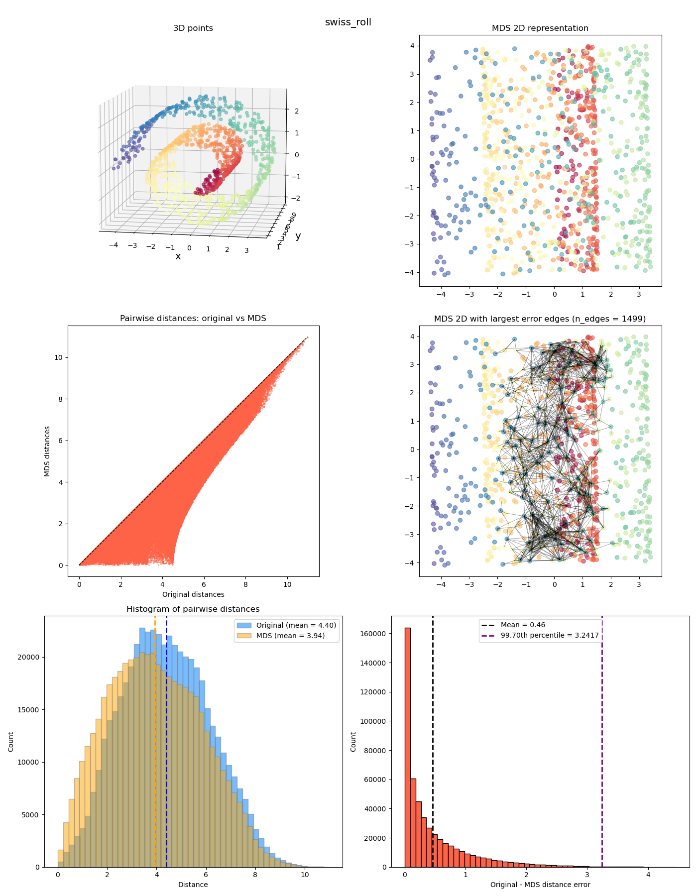
First, let’s start with a sanity check to make sure things are working:

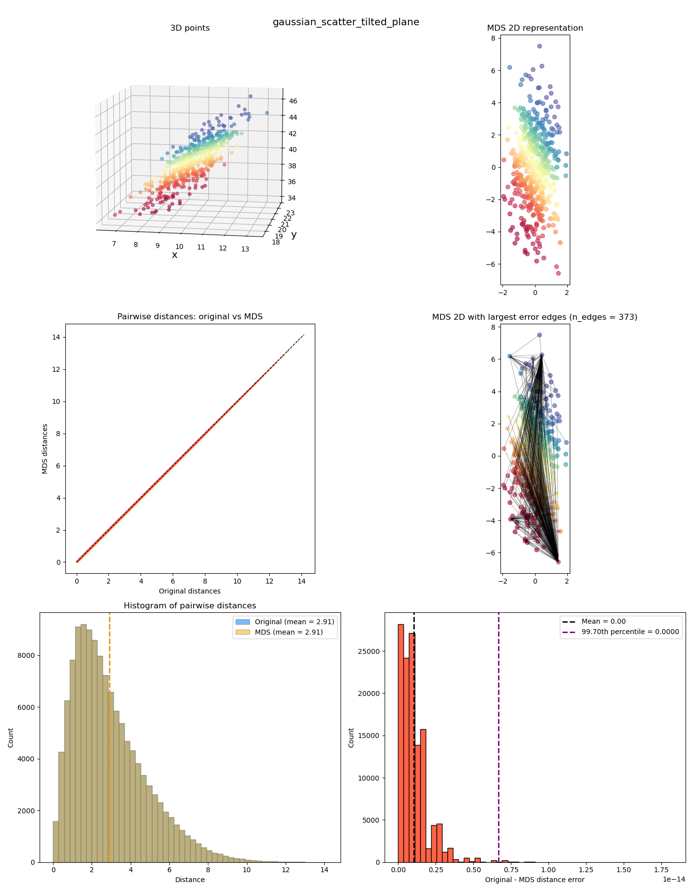
In the upper left plot are the “original” points in 3D space. In this first example, I’ve made a 2D Gaussian distribution but then tilted it with some slope (and colored it by its $y$ value). Since it’s inherently 2D planar, this means that we should be able to represent the pairwise distances perfectly in 2D. If this doesn’t work, we’re really screwed!

In the upper right plot are the 2D coordinates after the MDS transformation (with corresponding points colored the same).

In the middle left plot is a scatter plot with the “after MDS” vs “original” distances, so we can see how MDS distorts it. In this case, it’s perfect, so it’s basically on the diagonal line.

In the middle right plot, we have the same points as the upper right plot, but I’ve also plotted the edges that have the highest errors from the original distances.

In the lower left plot, I’ve plotted the before/after histograms of the distances and their means (again, perfectly overlapping in this example). And in the lower right plot, a histogram of the (absolute) error per point between the before and after (with the mean and percentile cutoff value for the edges in the middle plot). You can see in this case that it’s effectively zero; I’m guessing it’s not exactly zero because of some numerical stuff from finding the eigenvalues/vectors?

Anyway we can look at a few more interesting ones now:

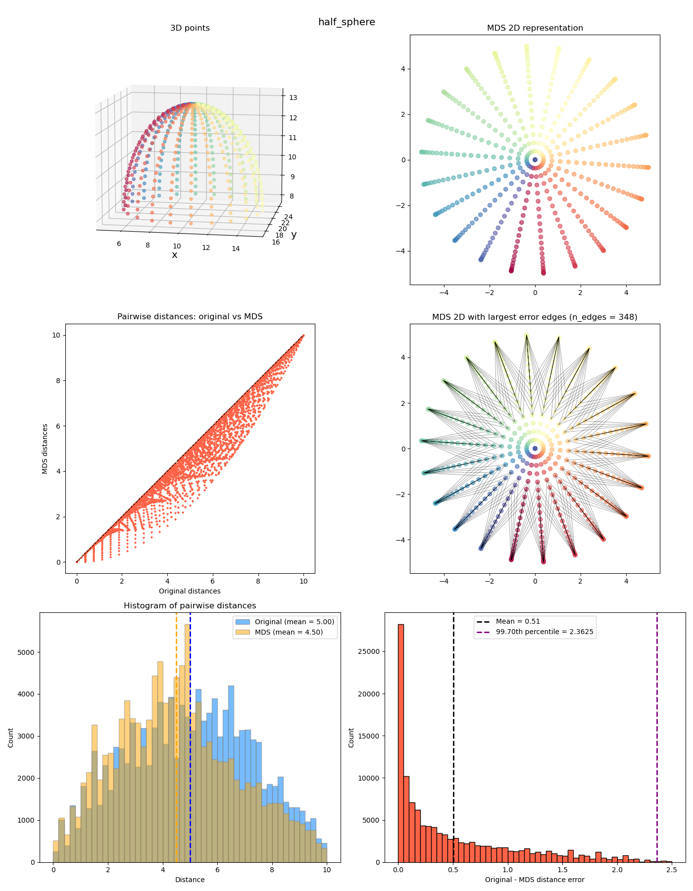
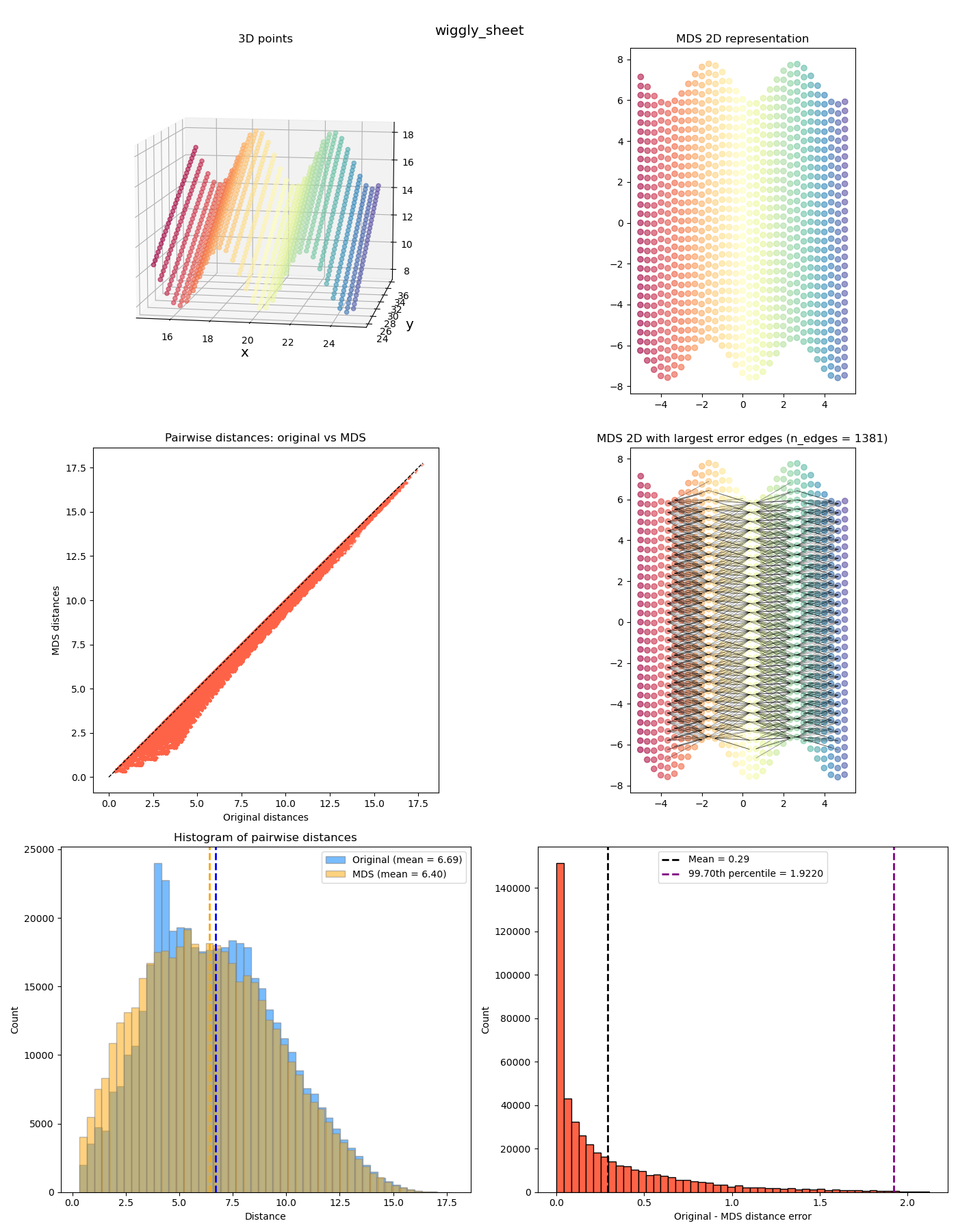
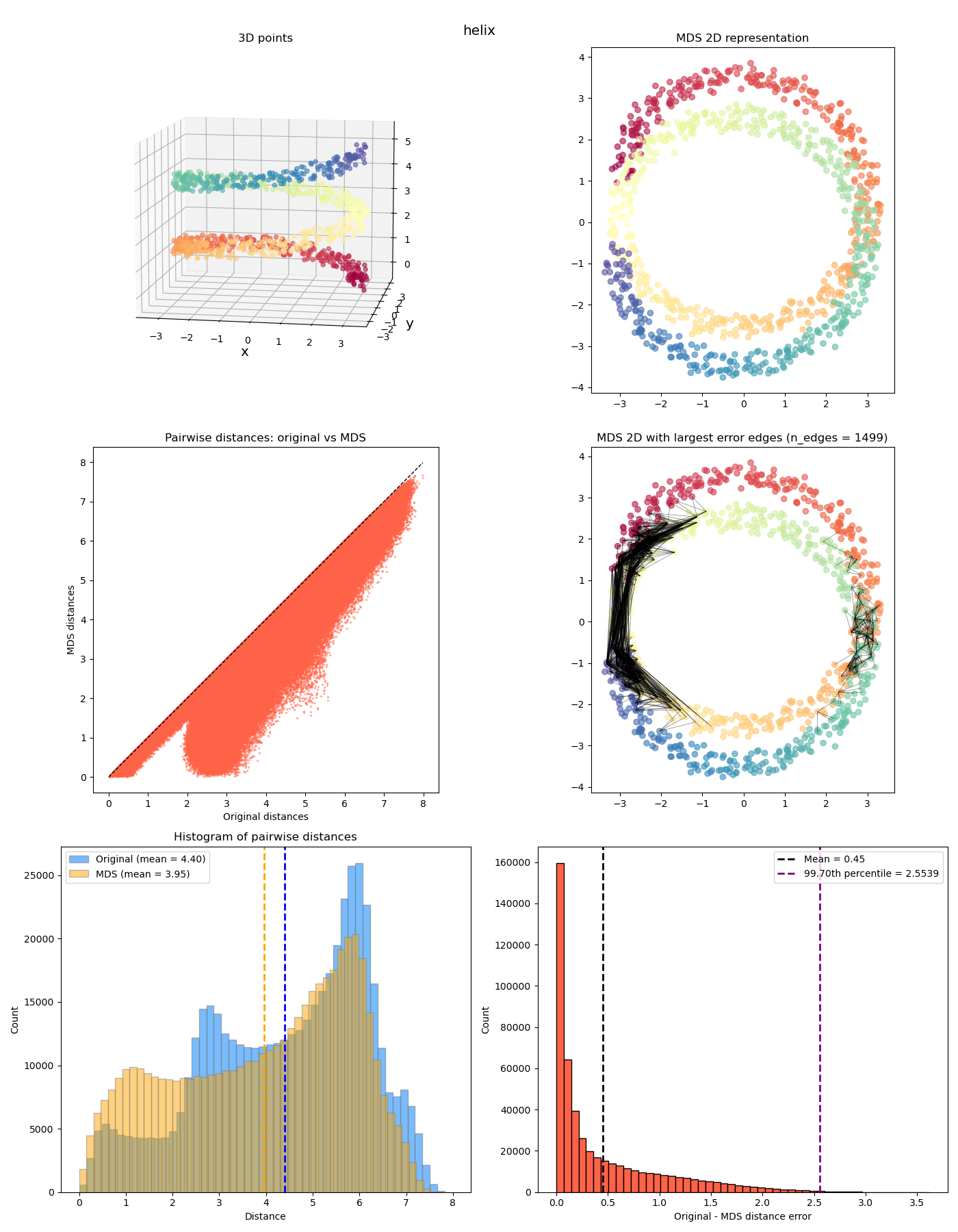
The last two feel a bit different from the previous ones. While the MDS coordinates from the previous ones could be gotten from the original coordinates by continuously “smooshing” / stretching the points down to the plane, in a way that’s (theoretically) invertible, the last two also smoosh them down, but they end up with points at different $z$ values getting smooshed to the same location, so it’s not invertible. It has a “quotient space” feel to it. More on this one in a future post!

Errata

Can you “predict” the coordinate for a new point without having to redo the whole thing?

You sure can buddy! To be concrete, our procedure was basically:

• we have $n$ samples and want to embed in $m$ dimensions
• we have the $n \times n$ pairwise distance matrix $D$
• we do the MDS procedure, yielding the $n \times m$ coordinates matrix $X$

Now we have a new point, $p_\text{new}$, and a vector $d_\text{new}$ of its (squared) distances to all previous points, and we want to find out how it’d get embedded in $m$ dimensions, i.e., its $x_\text{new}$ coordinate.

But… it’s not immediately obvious how. It’s not like in a linear regression problem where after the optimization you have the set of weights $w$, and then can predict a new point by simply doing $y_\text{new} = w \cdot x_\text{new}$ or whatever.

If you have a better memory than I did and remember back to your Bishop PRML chapter 6 on kernel methods, it’s pretty similar, since $B$ here is a Gram matrix. Here’s the handwavy answer.

First, we make a zero centered version of $d_\text{new}$: $\tilde d_\text{new} = d_\text{new} - \frac{1}{n} \sum_i d_{\text{new},i}$

then, we get what would be the new “row” in the Gram matrix for this new point by adding a vector of $B$’s mean across all entries ($\text{mean}(B) = \frac{1}{n^2}\sum_{i,j} B_{i,j}^2$) and subtracting the diagonal (vector) of $B$ :

\[b_\text{new} = -\frac{1}{2}\bigg [ \tilde d_\text{new} + \text{mean}(B) \cdot 1 - \text{diag}(B) \bigg ]\]

at this point, since $B = X X^T$, if $b_\text{new}$ were a row of $B$, it’d have the form $b_\text{new} = X x_\text{new}$, but this still can’t be solved for directly. However, we already have the $m$ eigenvectors/values from doing the procedure already, so we can just project $b_\text{new}$ onto them:

\[x_\text{new} = \Lambda_m^{-1/2} E_m^T b_\text{new}\]

Note, $b_\text{new}$ is an $n$-dim vector, as are each of the eigenvectors. So we’re effectively taking the dot product with each one of them (and scaling by the eigenvalue term too).

A pathological example

In a paper I read a little while ago on a related topic (kind of the reason for this post), they’re modeling (quasi)metrics, meaning they have a bunch of pairs of points, their distances, and want to build a model $d(x, y)$ that takes points $x$ and $y$ and outputs the distance from $x$ to $y$, in such a way that it has properties we usually want metrics to have, like obeying the triangle inequality, nonnegativity, etc.

A standard/simple approach is to make a mapping $\phi: \mathbb R^n \rightarrow \mathbb R^m$ (for example, a NN), and then define it as $d(x, y) = |\phi(x) - \phi(y) |^2$, i.e., training your embedding, and then using the Euclidean norm between the embedding of the two points.

This can work to some extent, but they have a very simple example that it’ll never be able to model with the Euclidean norm:

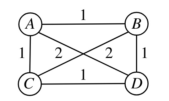
If you squint and scratch your melon for a while you can probably convince yourself that this is just inherently non-Euclidean: we want B and C to be 2 apart, which makes A and D both be at the midpoint of B and C, but then they don’t coincide, they also have a distance of 2.

Here’s its distance matrix:

\[\begin{bmatrix} 0 & 1 & 1 & 2 \\ 1 & 0 & 2 & 1 \\ 1 & 2 & 0 & 1 \\ 2 & 1 & 1 & 0 \end{bmatrix}\]

and here’s how the points get embedded into 2D with MDS:

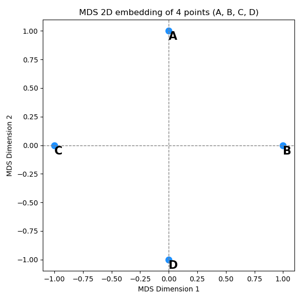
with distance matrix:

\[\begin{bmatrix} 0.00 & 1.41 & 1.41 & 2.00 \\ 1.41 & 0.00 & 2.00 & 1.41 \\ 1.41 & 2.00 & 0.00 & 1.41 \\ 2.00 & 1.41 & 1.41 & 0.00 \end{bmatrix}\]

You can see that it’s doing its best! The points have the $2$ distances in the right places, but it can’t quite do it all and has to “compromise”.

The key point here is: in the plots I showed above (for the example shapes), the distances had to compromise, but just because the data was inherently 3D, and we were forcing them to live in 2D. OTOH, in this example it had to compromise, but not because it didn’t have enough dimensions to make all the distances stay the same! It just can’t be done.

In fact, we can instead embed them into 3D:

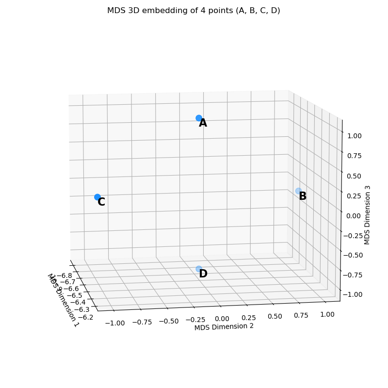
with coordinates:

\[X = \begin{bmatrix} 0 & 0 & 1 \\ 0 & 1 & 0 \\ 0 & -1 & 0 \\ 0 & 0 & -1 \end{bmatrix}\]

which you might recognize as basically the first plot with an unused extra dimension. And trust me when I say, the $d$ matrix for the embedded points are exactly the same too.

A data visualization tool?

I see why this could be called a data viz tool. But my small objection is that it makes me think of kind of… uhh, I dunno, “sleazy” methods like t-SNE. I say “sleazy” because a lot of data viz methods are either pretty uninformative and just look cool, or are actually outright misleading and often misused to show something that isn’t actually there. Even Wikipedia says:

While t-SNE plots often seem to display clusters, the visual clusters can be strongly influenced by the chosen parameterization (especially the perplexity) and so a good understanding of the parameters for t-SNE is needed. Such “clusters” can be shown to even appear in structured data with no clear clustering,[13] and so may be false findings. Similarly, the size of clusters produced by t-SNE is not informative, and neither is the distance between clusters.[14] Thus, interactive exploration may be needed to choose parameters and validate results.

That “interactive exploration may be needed” also has me nervous… “nah, that one doesn’t look as good. Change the seed a few times and rerun it!”