[latexpage]

If you frequently wander down the dark alleys of the computer science neighborhood of the internet, it won't be too long before you bump into a strange man in a trench coat who says "hey, kid... you ever try Functional Programming?" This man is not your friend. If you meet him, listen to him and do everything he tells you. It still won't save you, but it's for the best.

...I had heard the legends about FP, of course. The optimization. The ease of thinking about program flow. Learning Haskell will increase your height by at least 7 inches. Evaluation so lazy, you can't get it to compute if your life depended on it. Talking to simple humans will now require effort; their tiny pea brains can't comprehend the otherworldly beauty. Some FP coders have to wear special clothes because they start to grow small feathers.

Like most people, the first time I heard about FP was at a cool party, with many celebrities. I thought I heard someone behind me whisper some mysterious, foreign sounding word like "functor", and my ears perked up, trying to eavesdrop. However, they must have noticed, and immediately changed the conversation to the latest PEP.

When the "functor" person went to get another drink, I followed him to the kitchen. I was standing a little behind him and to side, and he was wearing a collared shirt, but appeared to have...gills? on his neck. I shook my head; the light must have been playing tricks on me. I approached him and said "h-hey... I heard you mention..something, back there?" His eyes flashed and he told me he had no idea what I was talking about.

It only took a minute of gentle cajoling before he was talking, more than I wanted and faster than I could understand. He told me that I didn't know purity and that I hadn't seen. He told me that the smallest program I could write "in java or whatever you cretins use" would still be larger than the largest program it's possible to write in Haskell. He was sweating, and the whites of his eyes had begun to turn jet black. He asked me if I had ever even heard of pattern matching, and told me that tomatoes and apples were the same thing. At this point, he appeared to be vibrating into a fine mist...

I don't remember much after that, but when I woke up the next morning my mouth was filled with sawdust. I coughed it out, got up, went to my computer, and punched in http://learnyouahaskell.com/.

 

Motivation and overview

I've been meaning to try out FP/Haskell for a while now. My friend Phil wrote a popular blog post/rant about why we should learn and use it, and I'm generally interested in things that have a cult-like following: either the people in that cult are a bunch of crazies, or the mothership actually is coming, and I wanna be on board when it does!

(This is a tribute to the delightfully crappy drawings at learnyouahaskell.com)

I was learning about Variational Autoencoders (VAE), and wanted to implement one to make sure I had the idea down and to mess around with it. Foolishly, I decided this was also a good opportunity to learn some Haskell. I've used enough languages for a while now that in general, it's not hard for me to practically use a new one after reading some tutorials and web searching. However, Haskell does... not have the same learning curve. For this project I kind of threw myself in the deep end, implementing a VAE and gradient descent with the Adam optimizer by hand (i.e., not using any backpropagation or deep learning libraries, just a matrix library). For the sake of my sanity, I produced all the figures in Python, from the output of the Haskell program.

I'll first talk about VAEs, then show my results with them using my Haskell VAE, and then talk about the many hurdles I faced in making it. Here's my adventure of building a VAE for my first project with Haskell!

 

Brief VAE background

I won't go too into the details of VAEs here, as there are a million tutorials for it (I'll post a few at the bottom). The theory in the Kingma and Welling paper that kicked them off is very readable. Here's the basic idea, using the typical notation: we have some data, $X$, and we're going to pretend that a very simplified model, $p$, generated it stochastically. This model has a latent variable, $z$ (a vector), that can take on different values, with probabilities $p(z)$. For a given value of $z$ it generates, the model can then generate data points $x$ with probabilities $p(x | z)$. So if you know the correct distribution of $p(z)$ and $p(x | z)$, you can generate data that's similar to/includes $X$. Typically, people choose the dimension of the latent space to be smaller than dimension of the data, because this 1) compresses the data, and 2) hopefully forces the latent space to learn a representation of the data that captures core features of it.

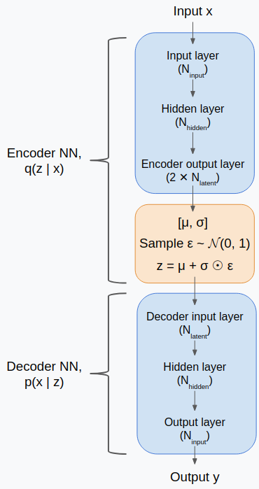
However, this is abstract. The actual goal is to approximate this model with an "encoder", $q(z | x)$, to translate data to that underlying latent space we're assuming, and a "decoder" $p(x | z)$, that lets you produce data from latent values. That's the general approach and could be done in several ways. However, a common way (and what we'll do here) is to approximate the model using a specific NN structure with two (or, depending on how you want to count it, three) main parts: 1) the encoder takes the input $x$ and transforms it into a vector of $[\mu, \sigma]$, 2) These are combined into the latent variable $z = \mu + \sigma \epsilon$, where $\epsilon = \mathcal{U}(0,1)$, and 3) the decoder takes this $z$ and produces the output $y$. More on the specifics of this below.

The loss term (see the paper for why this makes sense) is a sum of the "reconstruction error", which is just the MSE between $x$ and $\hat{x}$, and the Kullback-Leibler divergence between the prior $p(z)$ (which is usually taken to be $\mathcal{N}(0, 1)$ with the dimensions of $z$), and the encoder distribution $q(z | x)$. The motivation for the reconstruction error term is simple (we want to reproduce what we put in), but the KL div error is a little more opaque. It comes out of the math, but why does it make sense, intuitively? For a handwavy explanation, it penalizes the latent points for having less overlap with the prior. While incentivizing this will certainly increase your reconstruction error, you might want this. Forcing all the points to cluster more closely together could cause the latent space between and around latent points more meaningful, since they correspond to actual data points.

 

First experiment, MNIST digits

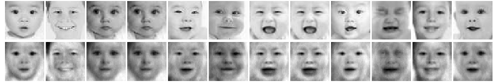
Let's start out simple. The classic you see with VAE (in fact, in the original paper!) is compressing the MNIST digits. The MNIST digits are 28x28 pixels, or a 784 digit vector. I'm using only one hidden layer of 1000 units in each of the encoder and decoder NNs, and we can actually squeeze them all through a bottleneck of 2 latent variables!

For example, here are a bunch of digits with their input image on top and reconstructed output image on bottom:

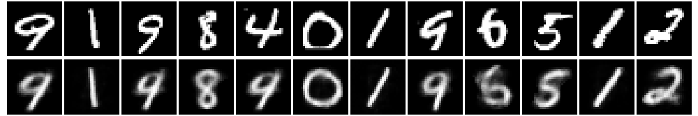
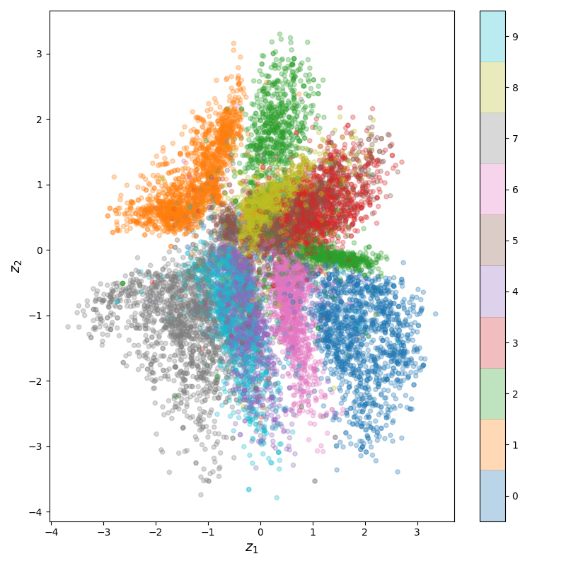
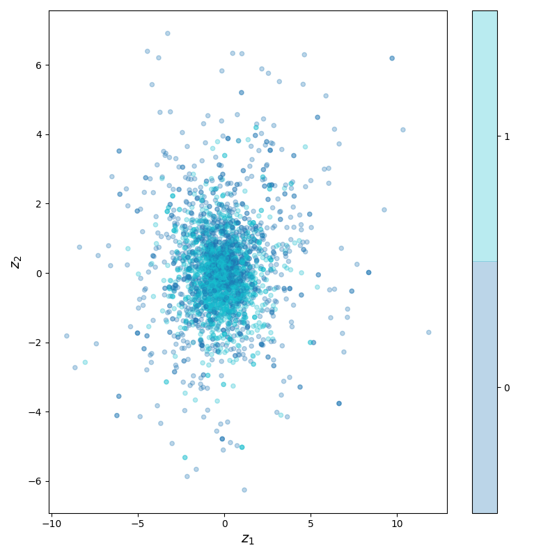
Obviously, they're not perfect, but it always impresses me that you can get that good reconstruction from two numbers. If you use a larger latent space, you can more easily get better reconstructions, but one of the advantages of using a 2D latent space is that you can easily plot the latent space itself! Here's what that looks like for MNIST:

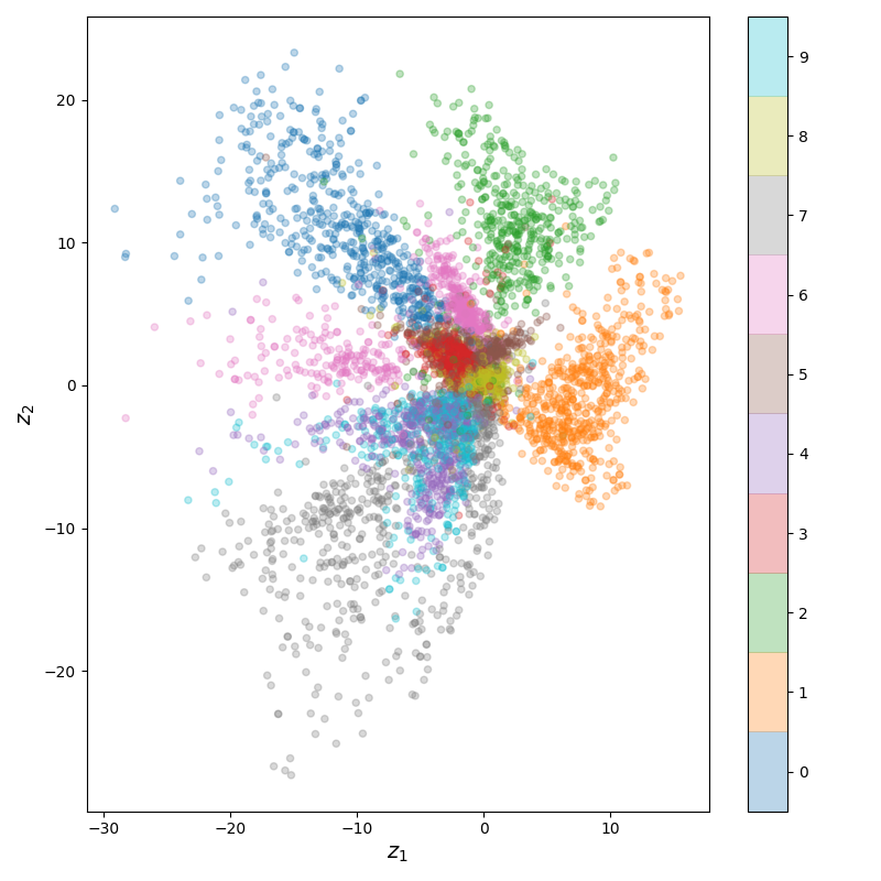
You can see that the clusters for the different digits are placed and overlap in ways that make sense. For example, 3's and 8's are pretty similar for most digits, and 4's and 9's are so similar that their latent embeddings are kind of on top of each other. Lastly, here's the training error (batch size of 32; I didn't use a train set here):

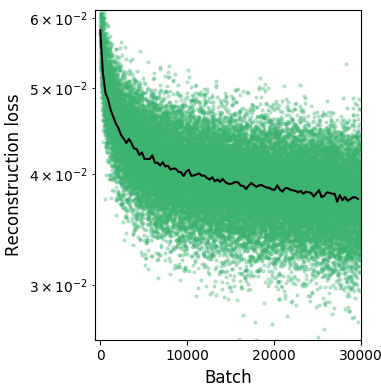
(Note the log yscale. Even though the returns are really diminishing, there's actually a noticeable difference in the reconstructed images halfway through vs the final point.)

However, I actually cheated here a bit. The loss is the sum of the reconstruction loss and the KL divergence loss. Typically, people use a coefficient I'm calling $\beta_{KL}$ for the KL divergence loss that determines how much to optimize it compared to the reconstruction loss. If you set it to 0, you've turned off this loss term and now you're only optimizing for reconstructing the input.

If you only want to recreate the input, then I guess this is fine. However, take a look at the latent space above. You'll see that the coordinates for $z_1$ and $z_2$ are pretty large! That's because there was no KL div loss, and the NN learned to make them large, as that allowed differences between different clusters to be more easily seen (i.e., keeping 10 distinct sub-distributions separate is easier in a 30 x 30 square than a 1 x 1 square).

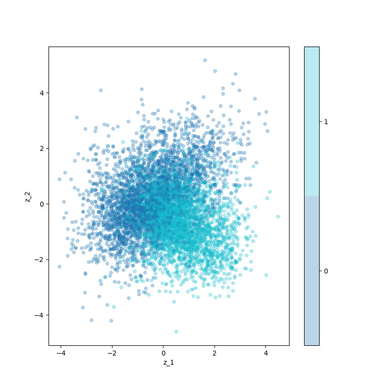
This has the effect that the space in between the distributions for separate digits doesn't have much meaning; $p(z)$ is low there and therefore if you try to calculate $p(x | z)$ from that region, you shouldn't expect it to look much like something from our data. However, if we choose $\beta_{KL}$ carefully, this has the effect of penalizing differences from the prior distribution, which is usually taken to be a zero centered Gaussian. Practically, this "smooshes" all the points in towards the center. Here's what that looks like:

Note the axes bounds, smaller with the pressure from the KL div. Now if we take a path from one point to another, we can see that it transitions much more smoothly:

We can also look at a little section of the manifold, by plotting the reconstructions of the points in a grid around a latent point:

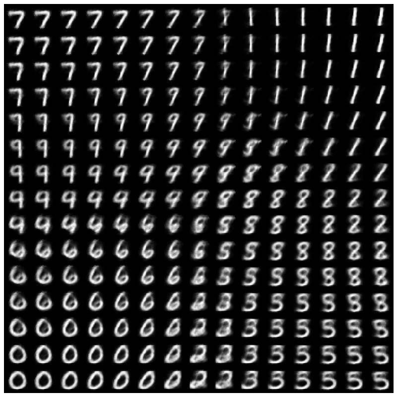
Neato!

Naturally, I wasn't satisfied. Everybody does MNIST! FP has given me an unholy and unquenchable thirst. Faces are another classic compression application. In the Andrew Ng machine learning course, he even has you do a fun assignment with finding the PCA of faces, and tons of people have done that with VAE, of course.

But...have people done it with dogs? and people? dogpeople? It's probably safe to assume that Jeff Dean has at some point, but I wanted to try anyway. Here's what I did.

 

Dogpeople

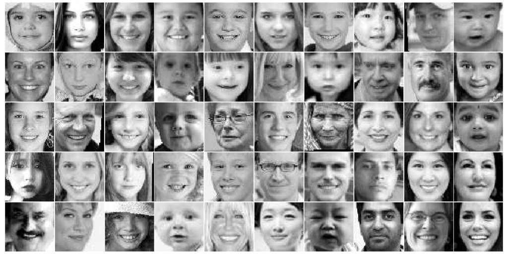
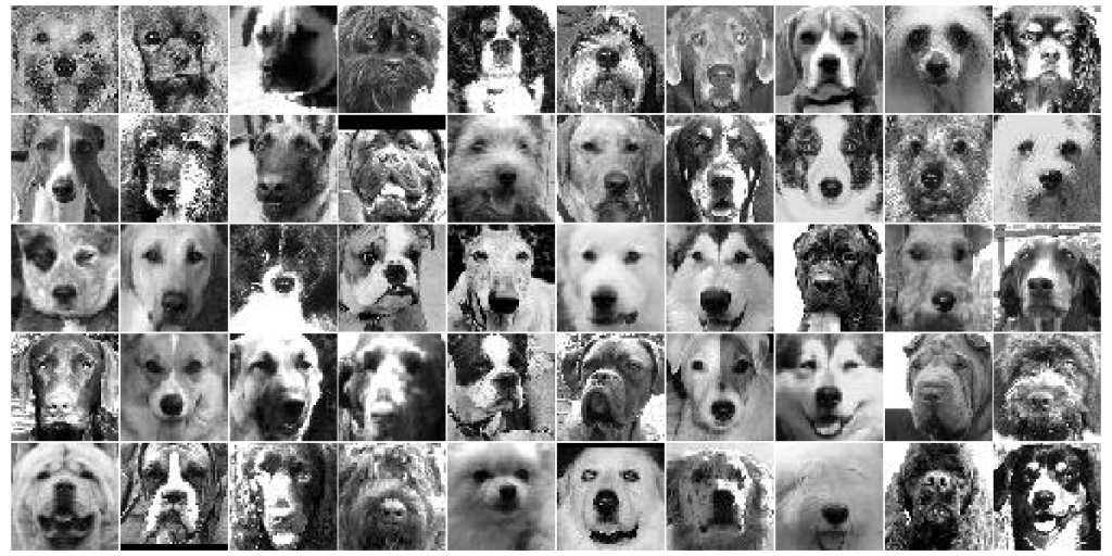
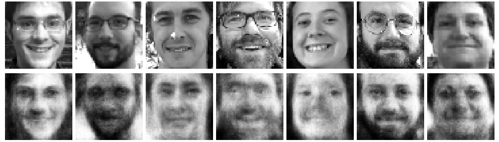
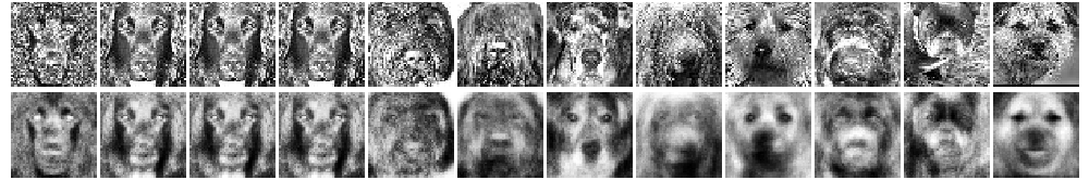
There was first lots of pre processing of the images, which I just did using Python, for my sanity. I found that both the amount of data and the way I set it up actually made a big difference! Datasets of human faces are pretty easy to find; I used the UTKFace dataset. However, dog faces are a little harder. There are lots of dog datasets, but not as many with specifically their faces. Originally I was using this Husky/Pug one, but Pugs have such god-awful faces that it was genuinely making it hard to learn. Additionally, there were only a couple hundred of them. I searched again and found the Columbia University "dogs with parts" dataset from this professor doing really cool stuff, which had a lot more, and even better, face landmarks! Maybe I'll cover that in a future post. Here's what a bunch of the processed human and dog faces I used for training look like:

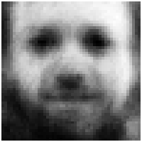
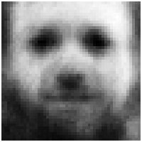
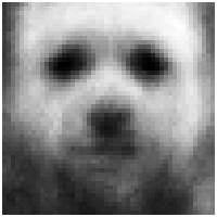
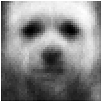
Onwards! So at this point I basically just had to train it, pretty similarly to MNIST. The first thing I found is that there's just noooo way it could encode meaningfully in two dimensions. Here's what that looks like:

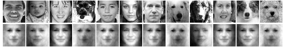
A couple interesting things. First, you can tell that the poor lil guy is really trying; it matches outline shades and a few other facets pretty well. Second, it's clearly encoding them all as humans, even the dogs. The dataset is half dogs, half humans, but I guess it found that with this constraint, it could minimize the loss more by just catering to reconstructing humans. However, from my brief experiments with this, I think this might actually just be a fluke -- I recall other times when it seemed like it was reproducing dogs a lot better than humans (when I was using a larger $N_{latent}$).

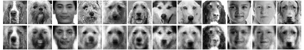
After experimenting a bit, I found that $N_{latent} \sim 50$ works pretty well for reconstruction:

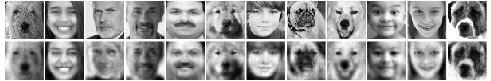
This isn't as big a compression factor as the MNIST above (784/2 = 392, 2500/50 = 50), but I think it also makes sense for a few reasons. First, MNIST digits are practically less than 784 pixels, since almost all of them have black pixels in the same positions (around the sides). Similarly, they're mostly black and white, while the photos use everything in between. Lastly, MNIST has 10 classes. It's not really clear what the "classes" with the dogs/humans are. It's obviously tempting to say "humans vs dogs", but there's waaaay more variation within all the humans than within one of the MNIST digits. For the dogs, they're actually sorted by breed, so you could call those classes, but again... once you count pose/contrast/etc, it's possible that those aspects make more sense as classes than the breeds. Sounds like something else for me to look at next time!

Like I mentioned before, since the latent space isn't in 2D anymore, we can't really plot it. Or can we?!? We kind of can. Here, I'm just taking the first two elements of the latent space and plotting them:

not much rhyme or reason obviously, because there's no reason to think those elements are very meaningful. I actually tested a bit with doing PCA on all latent embeddings and then choosing the components with the highest variation. It looked a little better, but still nothing like the nice ones for MNIST:

I wonder if this is because in a much higher dimensional latent space, the "clouds" of the data points can be in weird shapes, such that they look pretty overlapping when projected down to 2D.

Anyway, now for the fun part! Like before, we can transform between points. Now that we've gotten humans and dogs to reconstruct relatively well, we should be able to input a human, find its latent point, then input a dog, get its latent point, and decode a line of points between them. This works for any dimensional latent space, since we're just adding two vectors. All I'm really doing is this:

$x_{human} \rightarrow z_{human}$

$x_{dog} \rightarrow z_{dog}$

$z_{step} = (z_{dog} - z_{human})/N_{steps}$

$z_j = z_{human} + j z_{step}$

and for each $z_j$, getting $p(x | z_j)$.

Let's take it for a spin on my friends! First, let's try with Will.

Oh, sweet, beautiful Will. Won't you have this succulent Turkish Delight? om nom nom.

I dunno, Declan... I don't feel that good.

Don't worry, buddy.

What's..what's happening to me? 

What is it, boy? Are you trying to say something?

Bar bar bar! Bar!

Haha Will, you're so funny.

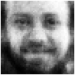
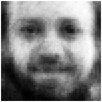
And here are some Cronenbergesque transformations of my friends!

Ben:

Bobby:

David:

Liz:

Max:

Phil:

Will:

These were with $\beta_{KL} = 0$, so it's purely reconstructing them. I tested with increasing it, but didn't notice any difference in the interpolations, but did notice a decrease in reconstruction quality.

I want to look into why it seemed to reconstruct my friends way worse than other images in the dataset. I didn't do much preprocessing to them, so it's possible they're different (like their dynamic range or something) than the dataset of faces I downloaded.

Recognizable when they're adjacent to their originals, but I'm not sure I'd recognize most of them without that prior. I didn't delve too far into this, but I wanted to see if they had much worse loss than typical samples in the dataset, so I plotted a histogram of the individual losses of a large number of samples:

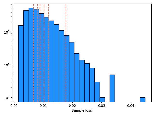
The losses of my friends are shown as the dashed lines. So they're mostly pretty average. I think what might be happening here is that, the big penalizer is broader features like shading/contrast/etc levels. So my friends' reconstructions have that mostly right, but what we judge it on are finer details like sharpness of facial features. I.e., we'd probably think an image that is 20% darker across the whole image, but in very sharp detail, is a better reconstruction than one that's much closer to the correct lightness level, but kind of blurry.

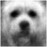
Lastly, I was curious: what are the images that reconstruct the best and worst in the dataset? Here's the best:

And here's the worst:

Interesting! Babies seem to get reconstructed very well, I'm guessing because they're pretty featureless here, and with a pretty flat lightness level. (As a quick aside, I think there's actually a biological basis I remember hearing about, that the young of most species look very similar to each other?) It seems like the dogs (and they're all dogs!) that are the worst have lots of speckling and detail in high contrast, which must both be hard to reproduce, and costly to the error when it misses it (for example, by trying the mean value between the two).

 

The Haskell battle

So far I haven't mentioned the Haskell part of this much, because I figured figures and results would be more fun for most people. Unfortunately, the above was relatively easy for me to learn/execute, and my main struggle was with some particularities of Haskell. So here's my adventure with that! I'll talk about a few big points and leave some particulars for another time.

VAE overview

Since we're essentially doing deep learning, everything is based on matrices. I based everything on the hmatrix package. It works pretty well for what I needed and has a lot of the same options numpy has, but its documentation is a bit weird. For example,  this Hackage page has some of its functions, but then there's this other page that has lots of useful functions I couldn't find on the first page. In addition, there's just not a ton of support for it online if you run into something you're stuck with. In addition, I believe you're stuck with 2D matrices. There are obviously NN packages, but I wanted to do things by hand to really get my hands dirty.

Structurally, the VAE is really two regular old NNs back to back, with a random sampling in between. However, while backpropagation is generally pretty easy to do with a typical feedforward NN, the sampling to calculate $z$ in between the two NNs make things a bit trickier.

I created a bunch of hierarchical types to make the code a bit more clear. I define that in a module like so:

newtype Layer = Layer {getLayer :: (Matrix R)} deriving (Show, NFData)
newtype NN = WeightMatList {getNN :: [Layer]} deriving (Show, NFData)
newtype Grads = GradMatList {getGrads :: [Matrix R]} deriving (Show, NFData)
newtype AdamOptim = AdamOptimParams {getAdamOptim :: (Matrix R, Matrix R, Int, Double, Double)} deriving (Show, NFData)
newtype NNAdamOptim = NNAdamOptimParams {getNNAdamOptim :: [AdamOptim]} deriving (Show, NFData)
newtype VAEAdamOptim = VAEAdamOptimParams {getVAEAdamOptim :: (NNAdamOptim, NNAdamOptim, Double)} deriving (Show, NFData)
newtype Batch = Batch {getBatch :: Matrix R} deriving (Show, NFData)
newtype VAE = VAE {getVAE :: (NN, NN)} deriving (Show, NFData)

A Layer is just a pseudoname for a Matrix R, to make its specific role more clear. A NN is a list of Layer, and a VAE is a tuple of two NN. I'll get to the others later! So, we'll mostly be passing around and modifying a VAE type.

Purity and IO

I found purity pretty easy to understand, but I guess I didn't appreciate it for a little while. My first stumbling block was when I needed to generate random numbers for the sampling part of the VAE. I searched for it and was getting puzzled and frustrated as to why I couldn't just find a simple pure implementation of random numbers. It took me embarrassingly long to realize that, if they're actually random, it isn't pure anymore; you won't be getting the same outputs for the same inputs every time. This really made it click for me: once the program is in "impure" land, you can still use pure functions and they'll act purely on their inputs, but your program as a whole is necessarily "tainted" by the fact that somewhere you let something impure in. Huh, the language gets weird with this stuff.

Lazy evaluation

This was by far my biggest roadblock. First, let me say: I think lazy evaluation is a cool concept! I see its merits and I'm sure if it's already on your radar, it's rarely a problem. That said, sweet JEEBUS it can really mess you up if you don't know where to expect that it might cause you trouble. I even knew about the concept of it when I hit this hurdle, but it was just so counterintuitive to me that it took a long time to figure it out. However, it's also very possible that I just set things up stupidly and I wouldn't have had this problem if I had done it the right way (please let me know if this is the case!). I'm not complaining about Haskell here, but it sure is a different way of thinking (which, to be fair, is what I wanted from this).

Really quick intro in case you're not familiar: lazy evaluation can basically be translated as "don't evaluate expressions until you absolutely have to".  What does "have to" mean, though? I think for most people, intuitively, if you have an input x = 5 and apply a function to it, y = f(x), and then another function to that output, z = g(y), they mentally picture calculating y and then using that to calculate z as soon as you declare z = g(y). However, in Haskell, it's more like, when you declare x = 5, y = f(x), z = g(y), you've set up the "pipeline" or "recipe" for calculating z but you don't actually have a value for it yet! And that's fine: if you don't actually need the value of z, then why should it waste time calculating it? Now, if you do something like print z, there's no way to avoid it: it needs to figure out the value of z to show it to you. So it would finally calculate z only then, when you did print z, even if that was waaay later in the program than when you declared x = 5, y = f(x), z = g(y).

I think this is counterintuitive to most newcomers coming from other languages (like me), but it has a bunch of advantages you can read about here.  However, it has a downside, or at least a common pitfall, that they mention there as well. If you think about the example above, there's a tradeoff: it didn't have to calculate z immediately, but it did have to keep track of how to calculate z, i.e., z = g(f(x)), which is called a "thunk". This isn't a big deal in that example because it's just two operations. However, if it was a crazy long sequence of a ton of operations, over a ton of data, it'll keep that MASSIF THUNK in memory until it actually needs to calculate a concrete answer...

Which is exactly the problem I had. My basic program structure was like this: I had a VAE structure like I described above, which was passed to my train_epoch_vae function, where it would read in training data, calculate the outputs, do backpropagation, and use gradient descent to update the VAE. However, to train for multiple epochs, I want to repeat the process, but with new data and on the updated VAE. The way I thought to do this is using one of the "fold" functions, where the VAE is the accumulator. I naively ran off and coded it up, and it worked... but I quickly noticed that it could only do a few epochs and it was devouring my RAM worse than Chrome.

The actual solution I found isn't that complicated, but it was hard to figure out. You can see from the link above that this problem is easily solved with foldl' or seq, which force it to calculate, preventing the massive thunk from forming. However, I'm not actually using foldl' -- train_epoch_vae is an action because it reads from file, uses randomness, etc. The fold for actions, foldM, doesn't have a non-lazy version analogous to fold', though the link provides a way to define one. However... I tried that and it didn't seem to solve the problem, the RAM still grew. I can't say I know exactly why, though. I'm still figuring that out.

Searching more and asking around, I eventually got to this solution. I still use foldM, but I define a dummy function with train_epoch_vae that uses force, from DeepSeq.

let train_fn = \(cur_vae, cur_optim, cur_train_stats) i -> train_epoch_vae (force cur_vae) (force cur_optim) train_info data_info cur_train_stats i
(new_vae, new_vae_optim, new_train_stats) <- foldM train_fn (vae, vae_optim, init_train_stats) [1..(n_epochs train_info)]

This...forces the argument to evaluate, which solved the problem. However, it seems ugly as hell, and I get the vibe from Haskell that there's probably a much more elegant way to do the same thing. Let me know what it is!

Last thoughts

Anyway, I think that's enough for now. I'm glad I finally tried out Haskell, though I really only dipped my toe in. I implicitly used some concepts, but I don't yet really understand the advanced things that seem to be what make people love it, so I am curious about those. I want to see what the fuss is about the esoteric stuff!

The repo for the code is here. I'm sure it's wildly inefficient and messy, so please give me any pointers or critiques you have!

I'll probably do another post soon on a ton of details about this project, both the VAE and Haskell side. There's a ton of stuff I found along the way that I'd like to look at more closely, like:

• Different schemes for "warming up" $\beta_{KL}$
• The effect of using different sizes of VAE layers
• Better Haskell implementations
• Different VAE architectures (IAF and such)
• Different interpolation schemes

See ya next time!

Resources:

• Auto-Encoding Variational Bayes
• Autoencoder tutorial people love on the internet
• Everything on Rui's blog
• Tutorial on Variational Autoencoders