Top-down program synthesis with a REPL and reinforcement learning

[latexpage]

Program synthesis is cool!

I came to it in a roundabout way, but I wish I had found it earlier. What immediately appealed to me when I started learning about machine learning were ideas of how to scale things up and build more complex structures from simpler ones. A while ago I did a couple projects with Genetic Algorithms (which can leverage modularity through schemas), before becoming interested in explicit modularity and trying a couple things with neuroevolution. I've read a bunch of recent papers about creating and reusing modules (usually, smaller NNs suited for specific tasks, "mixture of experts" systems, etc). However, these felt like they were missing the mark for me.

From my reading of the literature, Program Synthesis (PS) seems to be having a bit of a revival right now, where people are leveraging powerful, yet somewhat theory-light "general solver" methods like deep learning, reinforcement learning, etc, with the more theory-backed, math-based PS ideas (traditional PS has lots of overlap with areas like optimization, search methods, type systems, and constraint satisfaction problems). I've read a bunch of papers in this area that really struck a chord with me. Here are a few favorites:

Inspiration

I particularly liked the REPL paper above, so I thought it would be cool to try the same idea, but using a top-down approach instead of the bottom-up one they used. Although what I did is inspired by it, the top-down vs bottom-up choice makes it have some crucial differences. They use their technique in two common PS domains: text editing, and constructive solid geometry (CSG). CSG is essentially a set of "primitives" (shapes), and operations on primitives, that can be used together to create more complex shapes (a context-free grammar, to be exact). They also do CSG in 2 and 3 dimensions, but I only do it in 2D. Primitives and operations on them get rendered to create a 2D "canvas" (see below).

To appreciate the differences, here's a basic overview of their algorithm:

Each episode, a "spec" (goal canvas) is given
A collection of canvases that have been built up over the course of the episode is maintained
At each time step, input the collection and spec into the policy
The policy chooses an action that either adds a primitive, or combines canvases from the collection, to modify the collection
It also maintains a population of these collections (much like in an evolutionary algo), and uses its value function to determine which of them to continue expanding vs culling
If, at any point, it produces the spec canvas, the episode is over and it gets a reward of 1.

This is optimized using supervised learning (SL) pretraining (PT), and reinforcement learning (RL). RL has attractive features (despite its many, many pitfalls :P). For example, SL needs a label (i.e., a "correct answer") for a given task, but for RL, only an accurate scoring mechanism is needed. This can be useful when you either don't know what the correct answer actually is, or there are multiple correct answers.

Overview

Before getting to some of my results, I'll first go over 1) the task, 2) the algorithm, 3) the policy, and 4) the PT and RL procedures.

Task

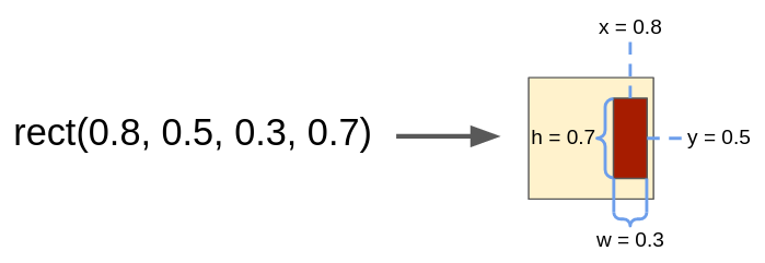
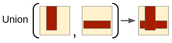
Each episode, a "spec" (goal) 2D canvas is given. This is just a 2D matrix, with elements in $[0, 1]$ corresponding to pixel values, where 1 is "display". A primitive is defined as a 4-tuple of floats, corresponding to the coordinates of a rectangle to be created on a blank canvas; i.e., primitive_rect(x, y, w, h) returns a canvas with the elements that rectangle encompasses set to 1 and all other entries set to 0. There are also operations that take some number of input canvases and produce an output canvas; for example, the Union operation takes two input canvases and returns the canvas that's the union of them. The task is to figure out how to produce the spec in a top-down way, working backwards from the spec and figuring out how to create it using only primitives and operations on them. Eventually, all canvases must be created from a primitive.

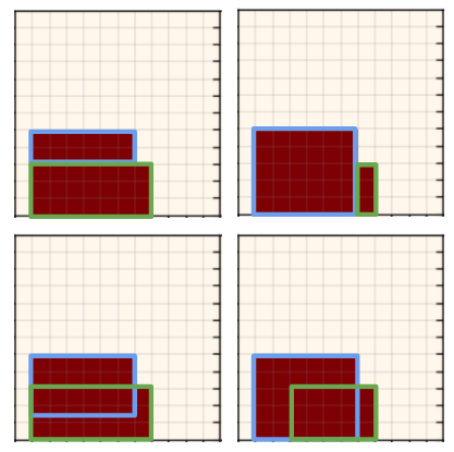
Typically the top-level spec canvas is created from several primitive canvases. Here are a few examples:

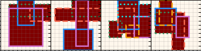
The primitive rectangles that each canvas is created from are highlighted in different colors, although all the algorithm "sees" is the canvas resulting from their union. Note that although each spec canvas is created from a specific set of primitives, many different sets of primitives could give rise to the same spec canvas (due to their overlap). More on that below!

Algorithm

Starting at a high level, the algorithm is as follows. The policy model, $\pi$, takes a canvas as input, and gives outputs that determine what to do, to reproduce the input canvas. The process is recursive; at each step, the policy either produces child canvases that it will also have to evaluate, or it produces a primitive, which is terminal for that call of the recursion. The end result is essentially a tree where leaf nodes are primitive canvases and other nodes are result of operations applied to their argument canvases.

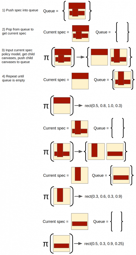
Here is the algorithm for a single episode:

A top-level spec canvas is given and is pushed into an empty evaluation queue.
In a while loop, until the queue is empty:
1. Pop the next queue element and feed it into the policy.
2. If the policy chooses to create a primitive, it creates a primitive canvas to match the input canvas, and the iteration is done (i.e., it's a leaf node in the synthesis tree).
3. If the policy chooses to do an operation like Union, it produces "child" canvases that are the arguments of that action. The child canvases are concretely specified but not built from primitives, so they too must be synthesized from primitives. Therefore, each child canvas is pushed to the queue.
When the queue is empty, the actual canvases created from primitives and actions can be constructed by "backing up" the tree, starting at the leaf nodes. Then, the actual canvases synthesized can be evaluated with respect to their spec canvases and rewards can be assigned.

That's a little hard to understand without visualizing it, so here's an example episode of the algorithm, if the policy behaved perfectly:

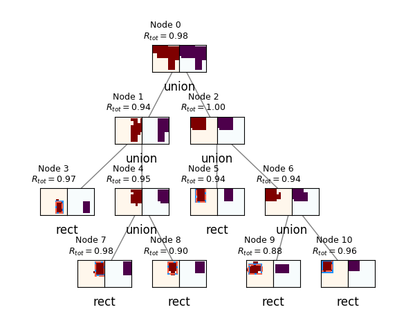
Once the queue is finished, you can assemble the canvases into a "synthesis tree" that shows how the original spec canvas is actually formed:

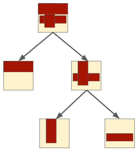
(Note that using a queue here means it's expanding them breadth-first, but because they don't have any dependence on order, depth first would give the same result.)

This describes how a spec canvas is built, but not how the process is optimized. Like the REPL paper, I also used a combination of PT and RL to optimize this process. See below!

Policy architecture

In describing the algorithm above, I glossed over the policy, although it's actually the thing that's being optimized. The policy model is separated into 4 parts:

The operation policy, $\pi_{op}$
The parameters policy, $\pi_{params}$
The canvas 1 policy, $\pi_{canv 1}$
The canvas 2 policy, $\pi_{canv 2}$

While these probably could have been combined into the same NN, I did it this way because it made it simpler to train and debug. Except for $\pi_{op}$, the other policies aren't necessarily used every step, since they're for different operations. Here's a block diagram of how the different policies are used for a single step from above:

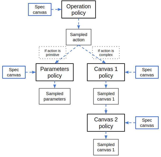
So the spec canvas is input to $\pi_{op}$ every step , and the operation to do is immediately sampled from its output and determines which of the other policies to use. If the operation was to create a primitive shape, then it will input the spec canvas to $\pi_{params}$ to create a primitive canvas. If the operation was a "complex" one like Union, then it will first input the spec canvas and a One-Hot Encoded (OHE) vector of the operation to $\pi_{canv 1}$, and use its output to sample the first argument canvas (for the given action). Then it will input the same spec canvas and the sampled canvas 1 it just produced into $\pi_{canv 2}$ to get the second argument canvas. Note that the same spec canvas is input into each policy, because each needs the spec to know what to do. I'll go over the policies briefly one by one.

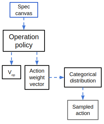
$\pi_{op}$ takes a spec canvas and returns a vector of softmax'd weights and a value function for that spec canvas. Because it's choosing a discrete action from a finite list, it just samples from a categorical distribution using the weights output by $\pi_{op}$.

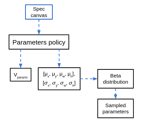
$\pi_{params}$ is used if the operation sampled from $\pi_{op}$ was a primitive operation. In that case, the same spec canvas is given to $\pi_{params}$, which outputs 4 values $(x, y, w, h)$, corresponding to the center $(x, y)$ coordinates, as well as the width and height of the rectangle to be placed. They go through a sigmoid before being output, so they're all in the range $[0, 1]$. These are transformed into the parameters for a Beta distribution, so the sampled values of the Beta distribution will be restricted to $[0, 1]$. The $(x, y, w, h)$ coordinates are all scaled to the canvas size so that 0 is the left or bottom, and 1 is the right or top, and $w$ and $h$ are the full width/height of the canvas.

When the rectangle is created, it's rounded to the nearest canvas coordinates, so it's discretized. Additionally, if the rectangle would go off the canvas area (by having a large $w$ and an $x$ near the edge, for example), it's clipped to only the section that is on the canvas.

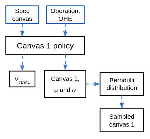
$\pi_{canv 1}$ takes the spec canvas as well as a OHE vector of the sampled action, and outputs a 2D matrix of $\mu$ values in $[0, 1]$ corresponding to the probability of each pixel being "on" in the first argument of the action. To get a sample, a Bernoulli distribution is used (although I also experimented with using a Beta distribution, which required outputting a $\sigma$ for each pixel as well).

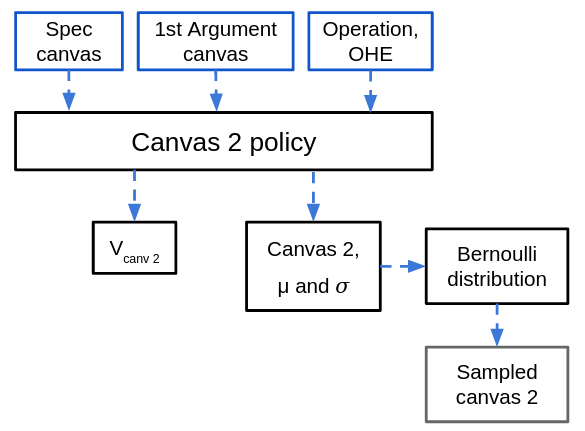
Last is $\pi_{canv 2}$. Here, it is given the spec canvas and the first argument canvas, which was sampled above (as well as the same OHE vector of the sampled action). Its output and sampling is of the same form as the canvas 1 policy.

PT vs. RL

Like the REPL paper, I did PT before the RL part. Because it's important, I'll briefly go over both parts.

While RL relies on returned rewards to figure out the right behavior, for PT we optimize the policy by directly maximizing the log probability of the correct actions. The PT optimization objective is almost the same as the RL objective, though the way we go about it is different. To be a bit handwavy, policy gradient RL is basically maximizing the expected accumulated reward by sampling actions from the policy and maximizing the log probability of the actions taken, scaled by their corresponding rewards (or returns, advantages, etc):

$$\nabla_\theta J = \mathbb{E}_\pi [R \nabla_\theta \mathrm{log}(\pi_\theta(a | s))]$$

However, part of the difficulty is that it needs many samples to figure out that the rewards it's getting from one action (in a given state even, not even counting other states) are more than the rewards from other actions, i.e., that it's the best action for that state. On the other hand, if you have the ground-truth best action $a_{true}$, you don't need to muddy the waters by sampling, and you can just maximize the log probability of that action:

$$L = \mathbb{E} [\mathrm{log}(\pi_\theta(a_{true} | s))]$$

(Note that while the policy gradient objective uses the expectation over $\pi$, I left the $\pi$ out of this one; the $\pi$ is in the PG expectation because the policy $\pi$ influences the distribution of samples it sees, but for PT, it's being given the same distribution of samples, no matter what the current state of $\pi$ is.)

In the REPL paper, they do a similar PT, but their ground truth samples are sequences of states and actions. In this project, because the synthesis is totally recursive, a sample is just a single step (of the algorithm above) and can therefore be optimized independently from other steps that might happen in a typical episode. Similarly, because the policies are completely separate in terms of what they do, they can be pretrained separately from each other. This turns out to be useful, because a couple of the policies get trained a lot faster than the others, per sample.

There's a bit of a trick I had to do here, specifically for PT $\pi_{canv 1}$. For $\pi_{canv 1}$, a spec canvas is the input, and if the operation is Union, the output should be a canvas that is a valid child canvas (that can be unioned with another child canvas to reconstruct the spec). However, a spec canvas is typically composed of several primitive canvases, so any of those should be valid outputs! Beyond that, even for a single one of the primitives, it can be completely ambiguous how far that primitive should extend into an area that's the union of several primitives. This makes things tricky, because for PT, we maximize the log probability of a single output.

To get around this, when doing the PT for $\pi_{canv 1}$, I input the spec canv, and take the outputs, which define the sampling distribution for canvas 1. Then, I evaluate the log probability for each one of the primitives that make up the spec canvas. I select the one that gives the highest log probability as the "correct" one (even though there are multiple!), and maximize the log probability of that one. This is a bit weird: it means that we encourage the policy to be more like the valid answer that it was already closest to. Also, it means the policy "collapses" to one of several valid choices. Ideally, it'd be able to sample all the valid choices for the same input, but I think this would need an architecture more like a VAE, where it samples in the middle of the NN, and then has more NN layers after that, before the final output (where it has to sample again). I think this would let it be able to output very different valid canvases for the same input. Let me know if there's a better way!

Anyway, doing PT is crucial for getting it to work. More on that below!

RL overview

This is one of the really interesting parts. RL is a way of optimizing behavior in a Markov Decision Process (MDP) where at each step, the agent is in a state, and can take an action that (stochastically) gives a reward and brings the agent to another state. However, because of the recursion/branching in an episode for this project, it's not immediately clear how to think about it in typical RL terms. For example, what is a state? It's tempting to say it's an individual spec canvas, but since applying the policy to a canvas can return two child canvases (like for a Union action), that would imply that an action can bring the agent from one state to two states, which I don't think makes sense in an MDP. I think a reasonable definition would either 1) view states as only single spec canvases, and say that an "RL episode" is actually just a single evaluation of that canvas, although the reward for the action can only be calculated after doing many of them, or 2) do something more complicated, like say a state is a collection of canvases (say, all the ones at a given depth in the tree). This makes more sense to me in terms of the state space, but it makes the reward allocation much less straightforward.

Anyway, I ended up doing something that's very similar to a typical policy gradient formulation, but with a few unorthodox modifications. First, recall that the actual policy model is 4 separate policies working together, which means having 4 different loss terms to optimize. $\pi_{op}$ gets used for every step, but the others don't always -- thus, the losses have different numbers of terms for the different policies across an episode or batch.

Second, while rewards from actions in later states are often accumulated and discounted to give credit to earlier state/action pairs, here I don't do that. The reward for a given action is simply the reconstruction score. However, this basically does have the effect of giving credit of future successes to past actions, because if the policy creates bad child canvases, they won't get reconstructed well, which will hurt the score at the current level. I actually did experiment with using a linear mix of the reconstruction score at the current canvas and the scores passed up from its children, but found purely reconstruction to be the best.

Notice that I also have a value function for each policy. The value function here can be easily interpreted as "the optimal score achievable given this canvas", which is exactly how I optimize it during PT. That is, a clean canvas should have $V = 1$, but if it has noise, it will never be able to produce the noise pixels, so it will have a slightly lower $V$. So why do I have a separate $V$ for each policy? Well, the policies are typically used sequentially, with the output of the previous one being the input of the next. Consider if the spec canvas was a perfect canvas for a Union operation, so $V_{op} = 1$. However, when it's input into $\pi_{op}$ to determine the action, if $\pi_{op}$ was badly optimized, or got unlucky and sampled "primitive rectangle", now when $\pi_{params}$ has to evaluate the spec canvas, it wouldn't make sense to say $V_{params} = 1$, because it can't possibly achieve that using a primitive rect. Therefore, the meaning of $V$ is more accurately "the optimal score given this spec canvas, provided you have to use this policy and any other inputs given to it". So it makes sense to "re-evaluate" (i.e., have a separate) $V$ for each policy.

Results

PT results

For PT, each of the policies are optimized separately. For a given policy optimization, the batch size is typically 32, but I record and plot the losses/etc of individual samples (across all batches) sequentially, which lets us see some useful info.

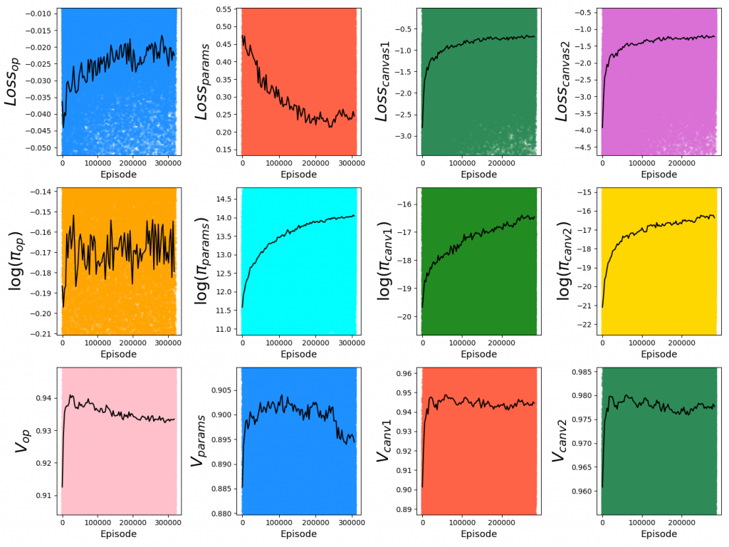
Below are PT loss curves for $2 \times 10^4$ batches, batch size 32, $N_{side} = 12$, hidden size = 1024:

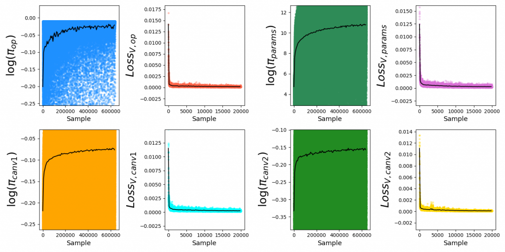
For each plot, each colored dot is the value for a single sample, while the superimposed black curve is a local average (to more clearly illustrate trends). You can see that it gets most of the improvement quickly, but the diminishing returns are actually pretty meaningful in terms of the scores they can achieve. Additionally, the corresponding value functions have much lower variance, since there's no ambiguity in their values (in contrast to the policies, which often have multiple valid answers).

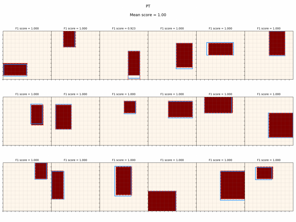
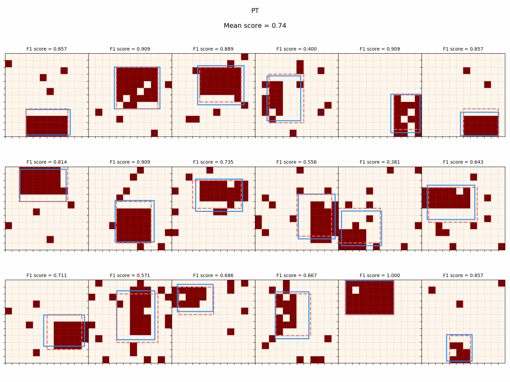
By plugging in a few example inputs to each pretrained policy, we can quickly get a sense of how well the PT worked. Here's what I've been calling a "primitive grid", where I plug a bunch of primitive canvases into the parameters policy and see how well the outputted parameters match it:

The blue outline shows the raw sampled parameters, and the dashed red outline shows the primitive that was "snapped" to the coordinates (that produces the actual canvas it would be judged by). You can see that PT optimizes this policy very well. Similarly, I test $\pi_{canv 1}$ by inputting a canvas produced by a complex operation:

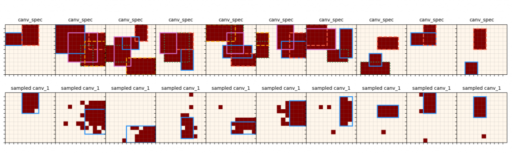
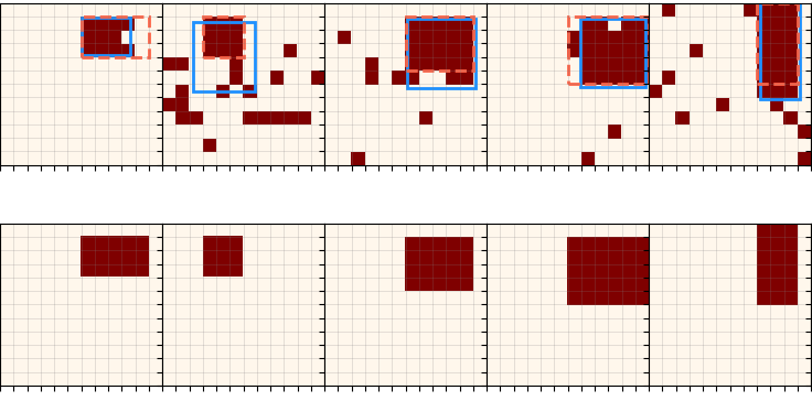
This shows the input canvas in the top row, and the corresponding canvas 1 that is output by $\pi_{canv 1}$, along with the outline of the primitive that it's closest to. Similarly, we can do the same for canvas 2:

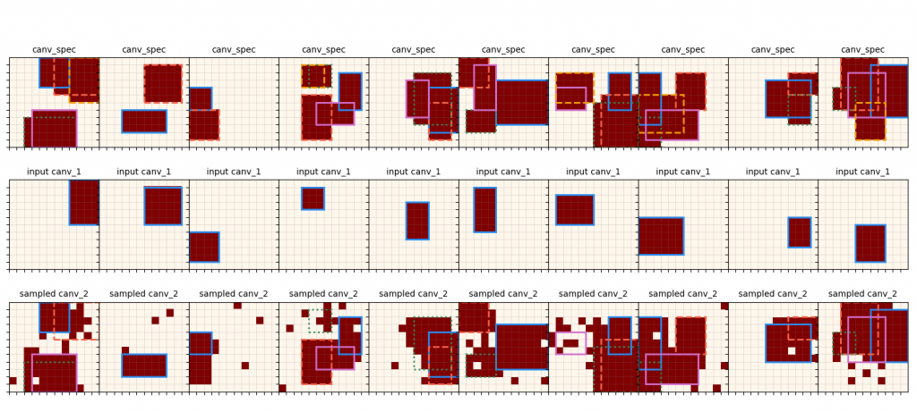
Since $\pi_{canv 2}$ takes both the spec canv, and the first canvas (that's already been produced by $\pi_{canv 1}$) as inputs, here I give it one of the primitives from the spec canvas as the first canvas argument. Note that these are much messier than the $\pi_{params}$ ones, since it has to optimize over a lot more ambiguity.

Let's go back to the PT curves again. Note that I've made it autoscale the y axes to the local average (black curves), but the actual range of the individual samples is much larger:

What's happening here? I made a function that looks out for and saves samples with a log probability below a specified threshold so we can inspect them.

$\pi_{op}$:

The top row is the spec canv that was actually given to the policy, and the bottom row is the ideal one (before noise was added). You can see that it's almost entirely due to $\pi_{op}$ choosing to do rect when it should technically be a union, but it often happens with canvases that are only a couple pixels different than a rectangle anyway.

$\pi_{params}$:

Here, the top row has the spec canv again, but it has the true rect in dashed red, and the one specified by the policy in blue. Again, the bottom row is the ideal canvas, before noise is added. There are some really clear examples here (all except the 2nd) of the noise messing up the shape so badly that it's basically closer to another rectangle...which $\pi_{params}$ then correctly finds! But unfortunately, it gets scored with respect to the "ideal" canvas. Of course, in practice, if it can match the noised one that well, that's great. The 2nd one there is a bit different, where instead of changing the rectangle to another, it seems like there just happens to be so much noise it messes it up completely.

RL results

Now, the RL results. While PT is relatively straightforward, there are a ton of variations and details to the RL part. The results below are for RL immediately following the PT above.

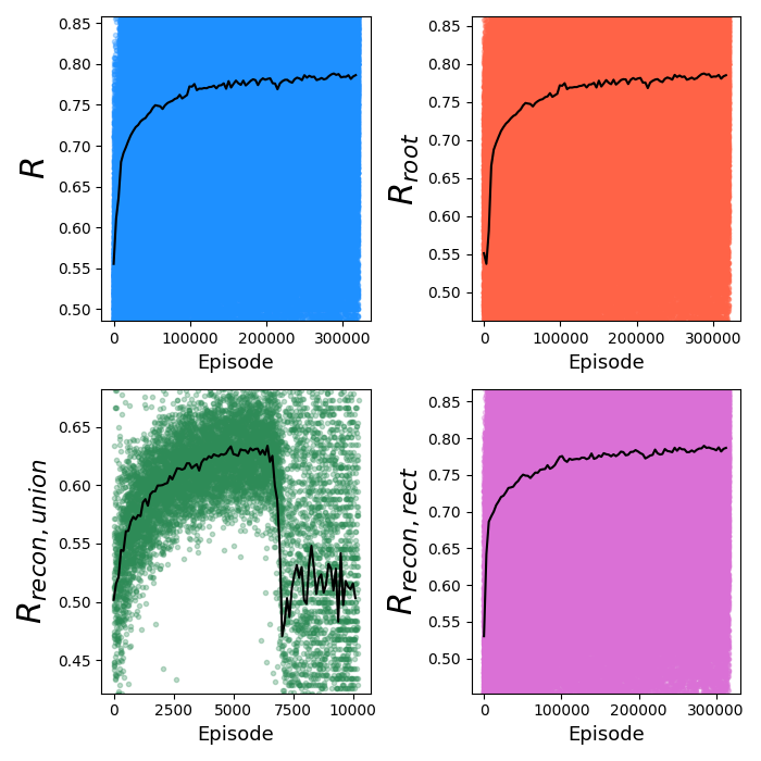
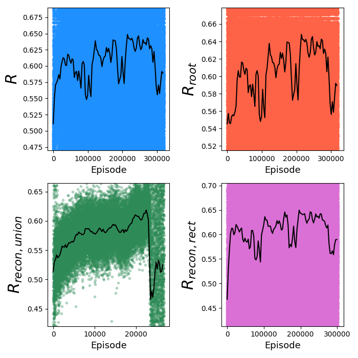
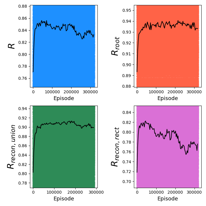
First, let's look at the train curves of the RL. Here are the most important, the reward curves:

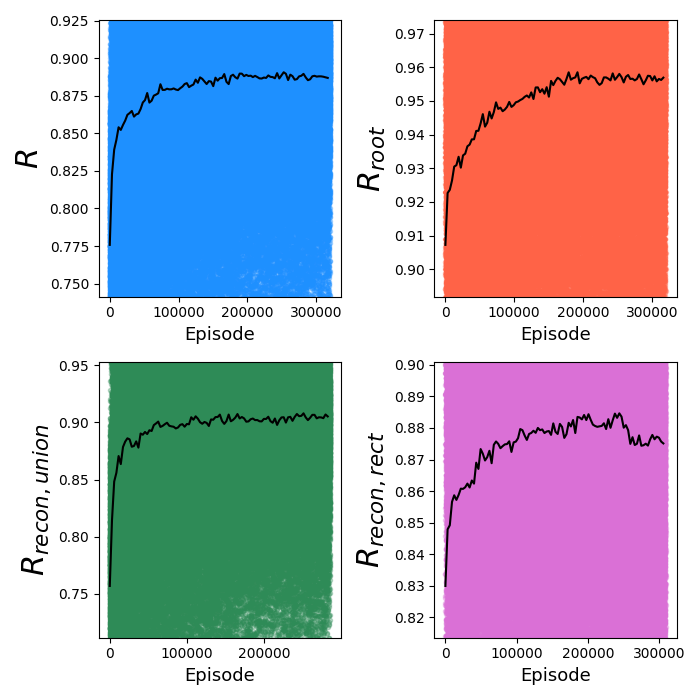
The most important plots are $R$ and $R_{root}$, because these are our main objectives. $R$ is the mean reward for an episode, across all nodes, while $R_{root}$ is the total reward for the root node of an episode. While $R$ is the actual objective that's being optimized for, $R_{root}$ is what we're ultimately interested in. Theoretically, if we could get a perfect $R_{root}$ score, we aren't concerned with the scores of the other nodes in the episode; however, typically $R$ and $R_{root}$ are closely bound because it's hard for $R_{root}$ to get a good score if its descendants don't do well either. Also note where the scores start: pretty high! This is because PT actually does most of the work, and even if it hasn't been optimized specifically for the RL episodes, it does a pretty good job for each canvas of the episode with just the PT.

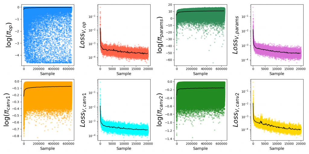
I also usually plot the log probabilities, V's, and losses of each policy, which look like this for the above:

However, for the sake of brevity (hah), I'll leave those out unless they're relevant.

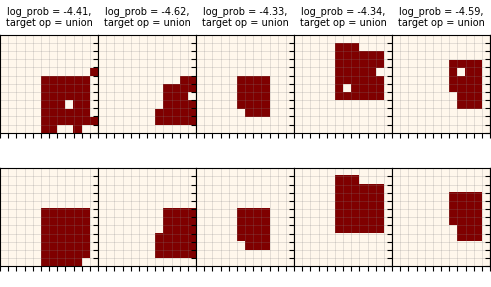
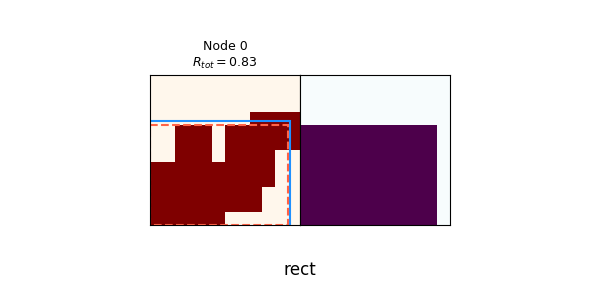
Lastly before I go into details and experiments, probably the coolest outputs are the actual synthesis trees produced by an episode! To do this, I just run an episode in evaluation mode, and save all the resulting canvases and rewards. Here are a few examples:

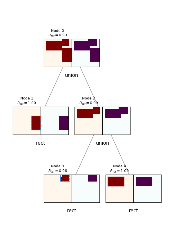
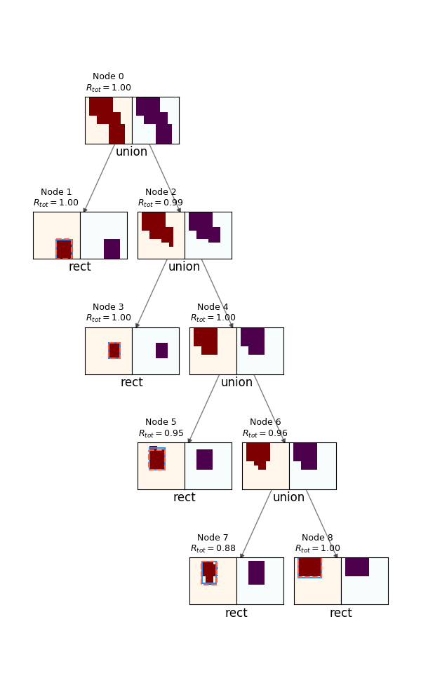
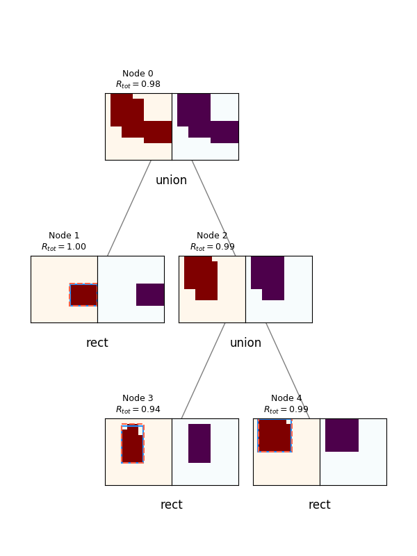
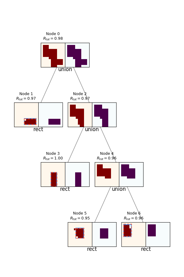
For each, the spec canvas is on the left, and its reconstruction (given its actions and reconstructions of its child canvases) are on the right. The node's number and $R_{tot}$ are displayed above each. You can see a few interesting things off the bat. It does a pretty good job, but it will frequently miss little corners if they're not large enough to register as part of an actual primitive, as opposed to noise. Also, note that although the canvases produced by the policy (canv 1 and 2) are often imperfect, because they get a primitive rectangle fitted to them, and the rectangle is what actually creates the reconstructed canvases, the root node is still able to get a perfect score.

Lastly, note the one in the upper right: it uses far more nodes than necessary (it can be created from only 3 primitives, but uses 5). This is a subtle point. I briefly experimented with adding a penalty to doing Unions, to prevent it from falling into a local minimum from "reward hacking" by just increasing the number of nodes. However (see below), the gains from using Union as opposed to just the best primitive for any canvas are pretty slim to begin with, so trying to dissuade it from branching unnecessarily this way is walking a fine line.

Experiments

How necessary is PT?

Since we're doing RL anyway, you might wonder how necessary PT even is: doesn't RL have the capability to learn on its own? Well, "RL has the capability" is a pretty weak guarantee. Even if it's technically possible for RL to solve this problem, it turns out that enough things have to happen simultaneously (across the different sub-policies) that it's extremely unlikely that it will happen with the random exploration that RL would have to do alone. For example, doing a successful Union operation depends not only on $\pi_{canv 1}$ and $\pi_{canv 2}$ producing decent child canvases, but also on $\pi_{params}$ eventually doing a good job.

Therefore, we should optimize with RL alone to see how necessary PT is. By default, the RL here is done using the advantage, $A = R - V$, to decrease the variance. I tested RL without PT in two ways here. First, doing the RL with the advantage, as is typical. Second, doing it only based on the reward, i.e., without subtracting the value baseline. The former is certainly attractive because it can significantly reduce the variance, but it also has the potential to mislead the optimization if $V$ doesn't get optimized carefully.

First, RL only, using the advantage:

Well, it does something, but definitely worse than with PT. We can see that it's pretty unstable, since $R_{recon, union}$ collapses after seemingly improving for a while. However, note the x range of that plot: they only go up to ~10k, while the others go up to ~300k. This is because in the $R_{recon, rect}$ and $R_{recon, union}$ plots, there are only points for each use of that operation, so this is telling us that the union operation is getting used way less often. This is confirmed by another metric that's always plotted, the $N_{nodes}$ for each episode:

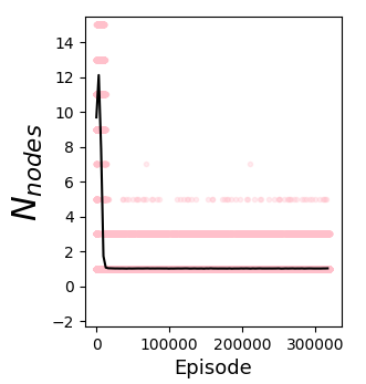
We can see that it quickly drops to $N_{nodes} = 1$, where it's trying to solve every spec canvas with a single primitive. Here are a few of the synthesis trees of that:

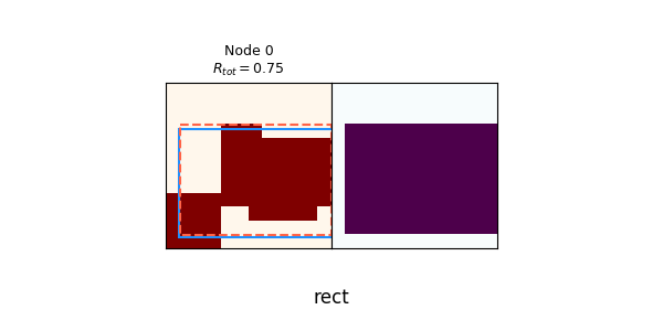
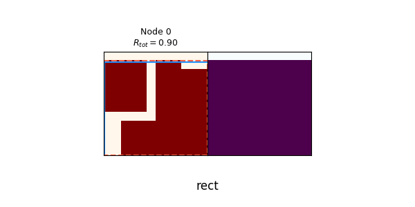
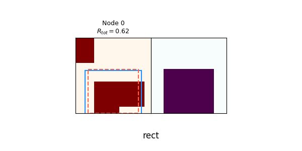
Given that it's only using primitive rects, it's actually not doing that badly! In the randomly chosen examples above, the worst one gets an $R_{tot}$ of 0.62, and the others get from 0.75 to 0.90. This is a prime example of why PT really makes a difference: RL can get these not-terrible scores relatively easily, but it's a local minimum. It briefly tries with more nodes at the beginning (i.e., using the union operation more), but the canvas policies are bad enough that they don't produce helpful child canvases, and thus $\pi_{op}$ learns that doing union is always bad! This could possibly be solved by enforcing exploration by adding an entropy term to the loss, but I didn't bother with that here.

Now, RL with no baseline subtracted:

This one does way worse, because it doesn't even have use of a $V$ baseline. Taking a look at the primitive grid, we can see that it doesn't even optimize $\pi_{params}$ well (let alone the canvas policies!):

Clearly, doing PT is huge. In fact, in the REPL paper, they even say they do "fine-tune with REINFORCE", implying that most of the work is done by the PT. I found the same!

How necessary is doing PT with added noise?

When I did a project on VAEs in Haskell, I briefly experimented with Denoising VAEs. I tried a similar thing here: when doing PT, instead of optimizing for inputs of perfect, clean canvases, I add random noise to the canvas in the form of removing a random mask of pixels, and adding another mask. Here's a typical example:

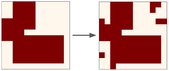
Why do this, though? Even after doing PT thoroughly, the policies which output canvases won't do perfect jobs, and will output canvases with minor mistakes. Therefore, we wouldn't want the policies to be very brittle to minor imperfections in the input canvases, which doing PT with added noise is meant to mitigate.

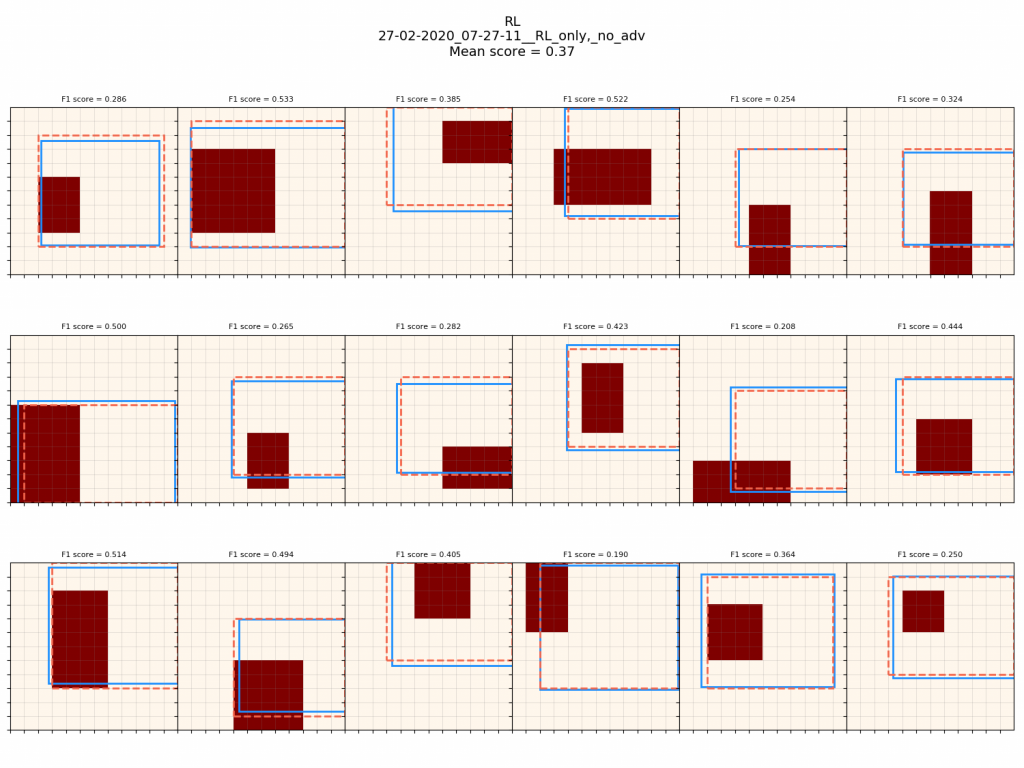
To illustrate this, let's look at primitive grids with and without noise, first with a policy that was PT with the default of adding noise during PT, and then with a policy that was trained only on noise-less canvases.

Policy with PT noise:

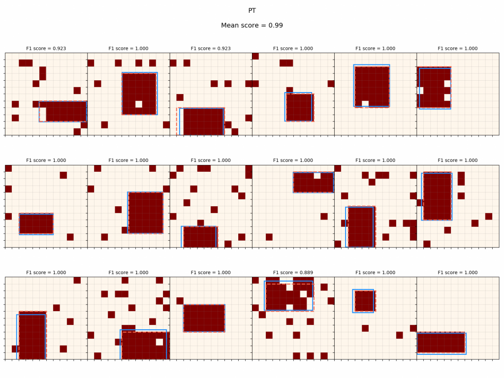
It gets nearly the same score when it has to deal with noise as when it doesn't. To be clear, the F1 score is with respect to the ideal canvas, i.e., how well it approximates the canvas before noise was applied (so it's not just penalized for doing a perfect job on a noisy canvas).

Now, the policy with no PT noise:

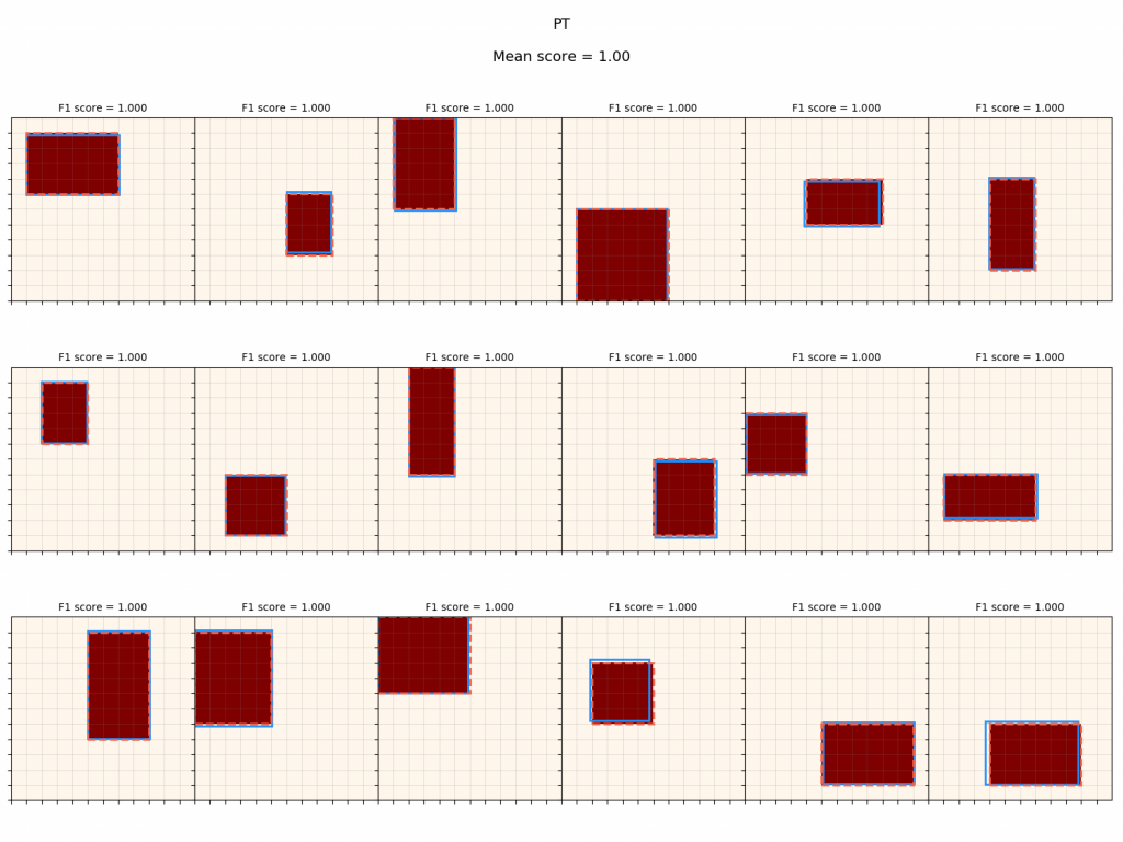
It gets hit pretty hard when it has to deal with noise, if it hasn't been trained to deal with it. Below are the training reward curves:

It seems like $R_{root}$ suffers a tiny bit (~2%) compared to the default version, and $R_{recon, union}$ is about the same, but $R$ is noticeably worse, and $R_{recon, rect}$ is much worse. I suspect that this is due to what I mentioned above when looking at the synthesis trees: although the reconstruction scores from primitive operations are worse, $R_{root}$ is relatively insensitive to imperfections further down the tree as long as they end up with their union covering the right spots.

That said, it seems like a pretty small gain overall. That said, I didn't experiment a ton with tuning the noise level: there's probably some optimal level where it pretrains the policy to be able to denoise most effectively, and I just tried a few things until it looked reasonable by eye.

Future directions

Anyway, that's all for now. There are about a thousand other details and experiments that I didn't get into here because it's already monstrously long. Here are some things I might look at in the future:

All the policies here were made from fully connected NNs, which are obviously pretty inefficient in terms of computation and number of weights used. I used conv NN's for a bit, which are the natural NN architecture for this project because the policy inputs are all images. They performed really well for $\pi_{op}$ and $\pi_{params}$, but were worse for $\pi_{canv 1}$ and $\pi_{canv 2}$. This is because while $\pi_{op}$ is doing classification, $\pi_{params}$ is doing something slightly different (but in the same ballpark), $\pi_{canv 1}$ and $\pi_{canv 2}$ have to output full canvases; they're basically doing image segmentation. There's of course a large literature on this, but I wanted to focus more on the algorithm and RL for this problem. In the future, I'd like to try using a Fully Convolutional Network or something.
I only used rectangle primitives here, but I'd like to have other shapes. I actually already built the machinery for this into the policies (which take an operation OHE input), but didn't end up doing it. One big reason is that a circle would have such low resolution on these grids that I suspect it would be difficult for the policy to reasonably recognize when one would be optimal to use. So this is related to the first point, where ideally I'd use a ~100 x 100 grid, where more detailed primitives could make sense.
Similarly, other actions: subtract, XOR, negate, etc.
Higher order operations, like duplicate/map.
As I mentioned above, currently, for a given spec canvas, $\pi_{canv 1}$ ends up being optimized to produce a single one of the valid primitive child canvases. I'd like to experiment with using architectures that can simultaneously produce different ones.

The code repo for this project can be found here. Please let me know if you have any questions, comments, or feedback!