[latexpage]

Skip to the full page interactive version if you don't want to read!

I made a post a while ago about recreating a Sol LeWitt piece using d3.js, and making it interactive. I had a lot of fun doing that one, and it wasn't even my favorite of his stuff that I saw! So, I knew I'd be back.

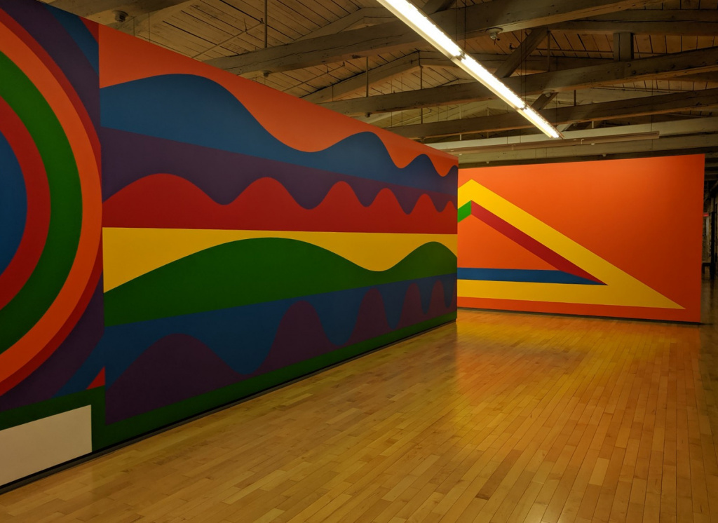
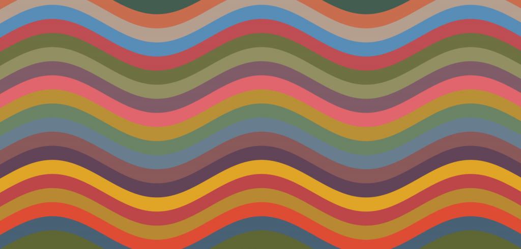
In some of his exhibits, he uses color in really great ways. The one I recreated previously didn't have a lot of color, so I wanted to do a really colorful one this time. It seemed like of the ones at MASS MoCA, the colorful ones could be divided into two categories: either really bold, primary and second colors, like:

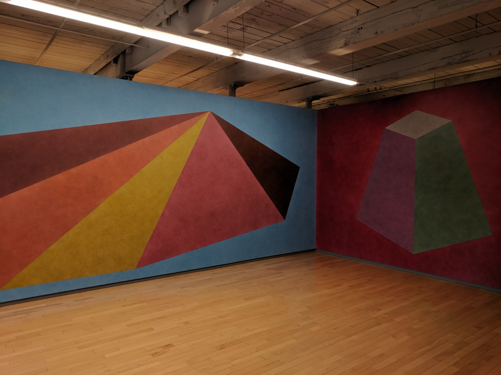
or, ones with more faded, more "complex" colors, like:

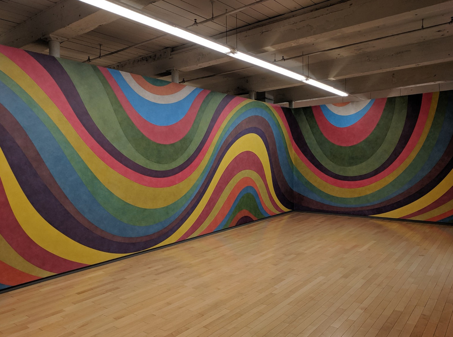
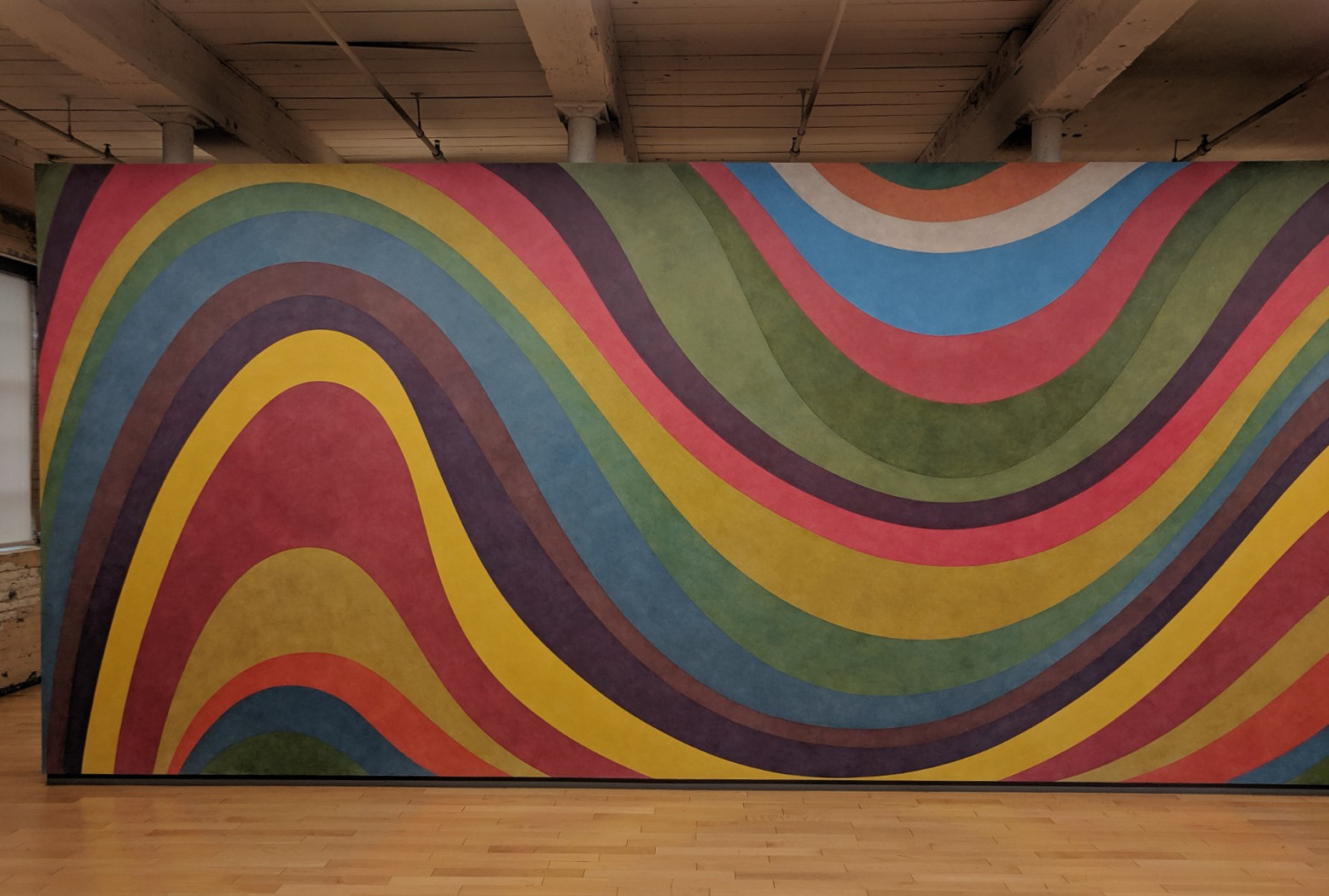
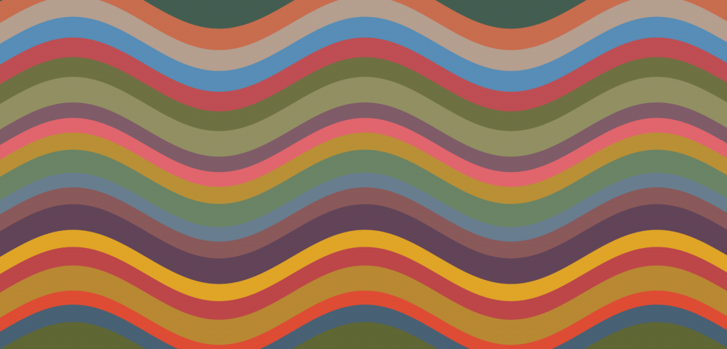
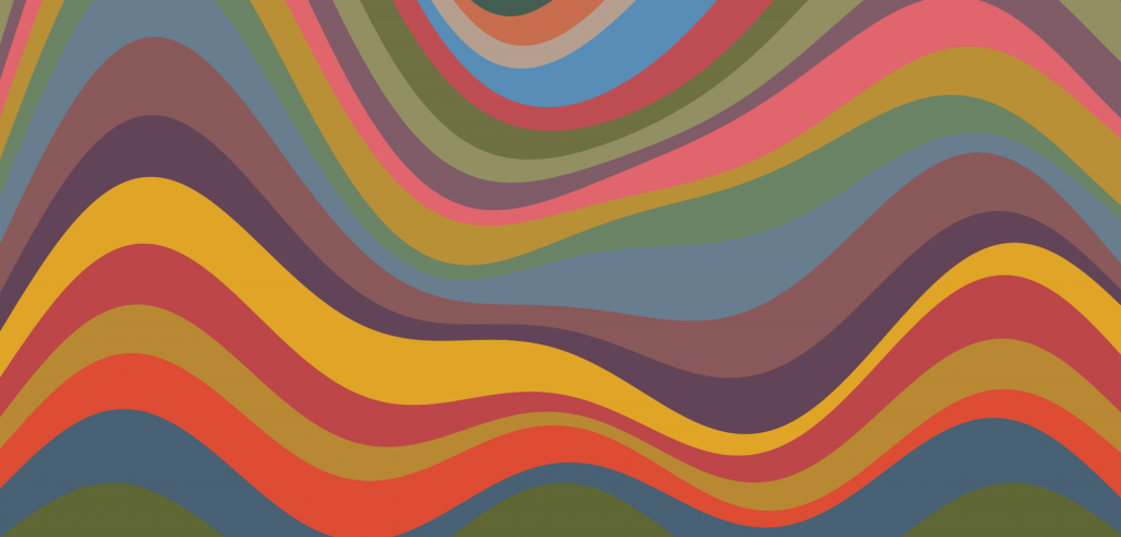
The one I'm doing today falls into the second category. Here are a few pics of it:

The basics of building it weren't hard, but the devil's always in the details. I created the basic structure using a d3 stack shape, and used GIMP to figure out the colors he used. Practically, this meant defining the "bottom" shape (a sine wave), and then adding layers on top of it; specifically, you choose the equation of the bottom layer, and then specify the thicknesses of the layers on top of it. However, if you simply do this with a bottom sine wave layer and constant thicknesses, you'll get a pretty boring result:

function sine_bottom_stack(n, m){

  var curves_stack = [];
  var pi = 3.14;
  var tau = 2*3.14;
  var f_0 = 1.0/m;
  var sine = [];

  // BOTTOM LAYER
  for (let j = 0; j < m; ++j){
    var A = 4;
    var f_mult = 2.5
    sine[j] = A*Math.sin(phase_0_sine + tau*f_0*j*f_mult);
  }
  curves_stack[0] = sine;

  // LAYER THICKNESSES
  for (let i = 1; i < n; i++){
    const a = [];
    var A = 0.6*t_band[i];
    for (let j = 0; j < m; ++j) {
      a[j] = 1.5
    }

    curves_stack[i] = a;
  }
  return curves_stack;
}

(n is the number of layers, m is the number of points used to define each curve. I do f_0 = 1.0/m to make the frequency you actually see on the screen be independent of the number of points you use to make the curve.)

Of course, there's a lot more going on in the real thing. The first thing is that it's obviously not a simple sine wave, it has some pretty funky variation.  For the sake of not having this be a huge wall of mostly repetitive code, I'll just use latex from here on out. $x$ is the position that the curve is determined by, $b$ is the equation for the base sine layer, $a_i$ will be the thickness of curve $i$, and I'll define other things on the way. So, what I have above is simply:

$ f_{mult} = 2.5

b = 2 \textrm{sin}(2\pi f_0 f_{mult} x)

a_i = 1$

The first thing is that the bands are obviously different thicknesses. To to this, I just made each $a_i$ a random term:

$ t_i = 1 + 1.2 \mathcal{U} (0, 1)

a_i = t_i $

where $\mathcal{U} (0, 1)$ is a uniform distribution. I'll leave the $b$ term as it is above for now, as we can get most of the interesting behavior by changing the $a_i$ terms. I'm including the $t_i$ here for reasons you'll see shortly. This gives:

Slightly better. The next pretty obvious thing is that they're not regular sine waves, they have variations across the length. To do that, I made $a_i$ have spatial dependence:

$ t_i = 1 + 1.2 \mathcal{U} (0, 1)

f_{band} = 2

a_i = t_i (1 + 0.6 \textrm{sin}(2\pi f_0 f_{band} x) ) $

Looking better! This is definitely the "Pareto jump" of this problem. However, it's still not quite there. The base thicknesses of each layer ($t_i$) are all different, and now each thickness is being modulated by position, which looks better, but they're still being modified by position by the same amount and in the same places. One easy way to change this is to add a phase term, $\phi_i$, that's constant for each band, but selected randomly for each:

$ t_i = 1 + 1.2 \mathcal{U} (0, 1)

\phi_i = 2\pi \mathcal{U} (0, 1)

f_{band} = 2

a_i = t_i (1 + 0.6 \textrm{sin}(2\pi f_0 f_{band} x + \phi_i) ) $

Hot daaaamn! We're getting there. That has the effect of making the modulation to $a_i$ just shift for each band, but it's still actually the same amount and happening at the same rate. Alternatively, we can do a similar idea, but for $f_{band}$ instead:

$ t_i = 1 + 1.2 \mathcal{U} (0, 1)

f_{band_i} = 1 + \mathcal{U} (0, 1)

a_i = t_i (1 + 0.6 \textrm{sin}(2\pi f_0 f_{band_i} x) ) $

DANG. In my opinion, that looks even better. And, together:

$ t_i = 1 + 1.2 \mathcal{U} (0, 1)

\phi_i = 2\pi \mathcal{U} (0, 1)

f_{band_i} = 1 + \mathcal{U} (0, 1)

a_i = t_i (1 + 0.6 \textrm{sin}(2\pi f_0 f_{band_i} x + \phi_i) ) $

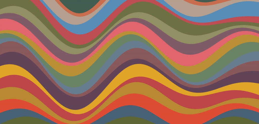
Now we're cookin.

At this point, the following were basically a bunch of little tweaks I did by hand, to taste. To make a long story short, at this point I adjust the base sine again. I make it have a larger amplitude, a few randomly sampled phases, an amplitude that varies with position, and a frequency that varies with position:

$ \phi_b = 2\pi \mathcal{U} (0, 1)

\phi_0 = 2\pi \mathcal{U} (0, 1)

\phi_f = 2\pi \mathcal{U} (0, 1)

A = 4 (1 + 0.3 \textrm{sin}(\phi_b + 2\pi f_0 x) )

f_b = 2.5 (1 + 0.2 \textrm{sin}(\phi_f + 2\pi f_0 x) )

b = A \textrm{sin}(\phi_0 + 2\pi f_0 f_b x) $

Note that this has the effect of making $b$ have a nested sine!

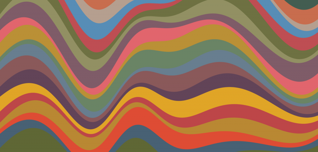
Pretty close to the main idea in my opinion!

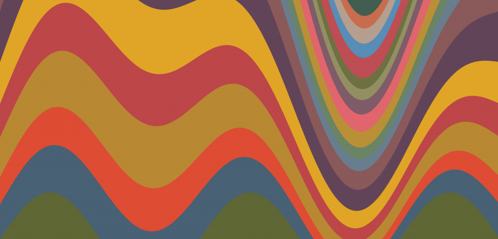
However, this is just one part. To make mine a little more fun, I wanted to have it be time varying. To do this, I made it so it periodically updates a few of the variables that should give some shape change, especially in aggregate. Each time step, it does:

$ C = 1

\phi_0 \rightarrow \phi_0 + 0.02 C

\phi_b \rightarrow \phi_b - 0.04 C

t_i \rightarrow t_i + 0.02 C \mathcal{U} (-0.5, 0.5)

f_{band_i} \rightarrow f_{band_i} + 0.005 C \mathcal{U} (-0.5, 0.5) $

I also wanted to make it so the user could control how much it changes, but not have them mess with actual numbers. To do this, I have it capture the current mouse position. There's a "band" in the middle of the window where, if the cursor is within that band, it won't change at all. Outside that band, it changes faster depending on how far outside of it you are (to the maximum at the edge of the screen). That's why that $C$ is up there! It's dependent on the mouse position. I'm curious if people will figure that out or not?

Another interesting aspect to this is that, due to how I'm updating $t_i$ and $f_{band_i}$ above, they'll act as random walkers: having average 0 change in value over infinity, but large fluctuations too.

There's one last aspect to this, and it was actually a doozy and pretty interesting. If you notice, in his painting, they're not solid colors, and it gives this really interesting "mottled" effect. My friend Bobby said that he read one of the plaques at the museum and it talked about the process, something known as "India washing" where they paint in layers, doing things to them in between. I really wanted this effect, but wasn't sure how to do it. I thought d3.js might have some clever way of doing it, but I couldn't find it despite my best Google-fu. I knew that what I wanted had to involve some way of randomly changing the intensity of the color, with some specified correlation distance (so it would have that "patchy" look and not just be seen as a uniform dimmer color).

I finally found a way, using a technique I didn't know about before: SVG filters. They're really interesting and I'll definitely be using them in the future, because they seem really powerful. Here, I'm using the feTurbulence filter, which uses Perlin noise, to create the mottled look. By itself, it looks like this:

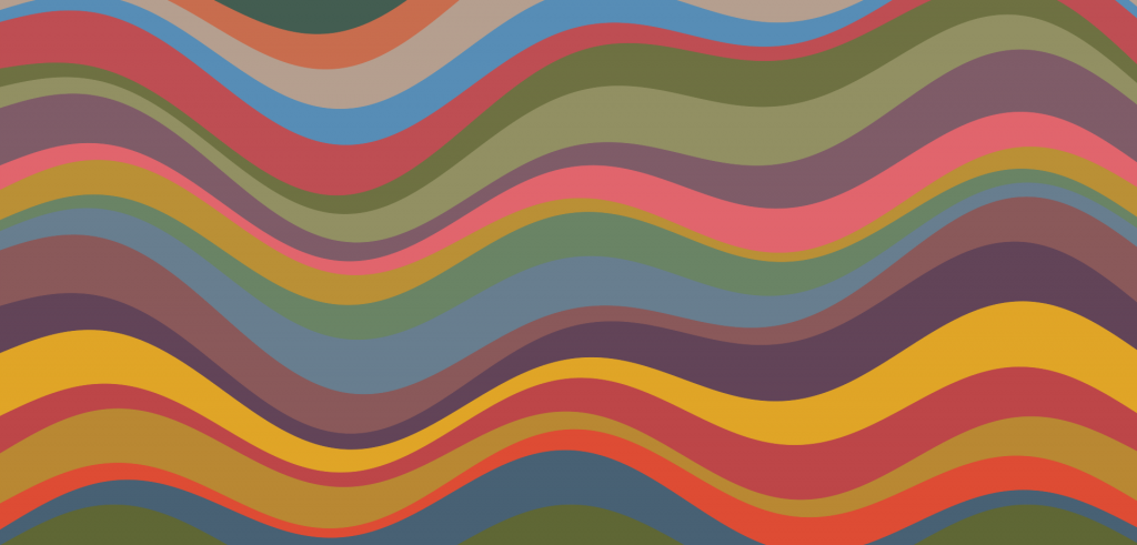
To use this, I had to employ a couple other filters. Filters are kind of functional in the sense that you can "chain" them together to make more complicated effects. First, I applied a grayscale to the above one. Then, I used the composite filter in xor mode to combine it with my svg of the bands. This makes it so where the noise filter is lighter, the colors will appear more, and vice versa, giving the mottled look:

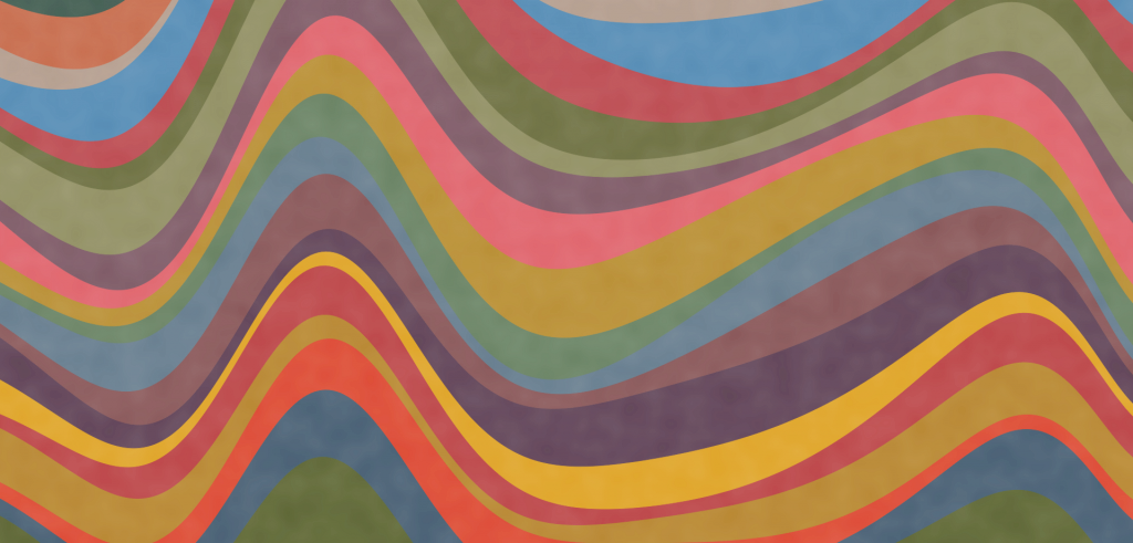
Ohhhhhhhhhhh yes.

One downside is that it's applying the same filter to the whole svg, so if you look closely, you can see when it moves that there's a kind of constant pattern "behind" the bands (or if you look closely when it's stationary, you can see some patches cross band boundaries). Ideally, I'd like them to each have their own noise pattern. I can do this, but when I tried instead applying the filter to each band, it was incredibly slow and basically couldn't move. I'm not exactly sure why this is. On the one hand, I know why it might be slow: it's just doing a pixelwise xor each time, which has gotta be intensive. On the other hand, it apparently does it fine for the whole svg. When I do it for each band, it's only doing it for the bounding area of the band. Maybe I'll figure it out someday, but for now it's a pretty diminishing return.

Anyway, here's the full, interactive version! Give it a try. If you like how it looks at a given point, there's a button to save the image! (without the button itself in the image :P)

It was tons of fun to make this and I'm sure I'll do it again in the future. d3.js is very cool and Sol LeWitt's works are perfect for it. See you next time!