[latexpage]

A while ago, this Numberphile video came up in my youtube feed. It's a cool little puzzle I hadn't seen before. Check it out! (because the rest of this post will talk about it :P)

It's not hard to solve if you think about it for a few minutes, but my first thought was that I wanted to do it with reinforcement learning (RL). There are obviously lots of ways you can go about it, but here's what I did!

 

Overview

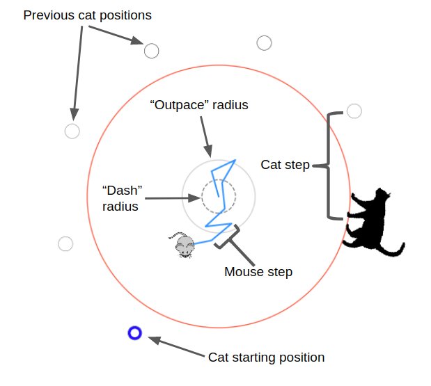
Very briefly, here's how I set up the mechanics of the problem: The cat is at the edge of the circle, which always has radius 1.0. The mouse always starts in the center of the circle, but the cat starts at a random position on the circumference. The mouse's speed is defined by the distance it goes in a time step, and I define that distance as some fraction of the circle's radius. The cat's speed is defined as a multiple of the mouse's speed, so I'll talk about $v_{cat}$, that multiple. Every iteration, the mouse takes a step in some direction to its new position. If it's not outside the radius, the cat goes in the direction around the circle that gets it closest to the mouse's new position, and the step is done. If it is outside the radius, we check if the angular difference between it and the cat's angle is less than or equal to the angular distance the cat can go in one step. If it is, the cat caught it and the episode is over. If it isn't, it escaped and the episode is also over!

I set up the reward structure so the mouse gets a reward of +1.0 if it escapes, -0.5 if it is caught, and an incremental penalty for each time step ($-1.0/N_{steps}$, where $N_{steps}$ is the maximum number of steps in an episode. I.e., it gets a reward of -1.0 if it never escapes or gets caught). So the reward structure is pretty similar to something like MountainCar, where it only gets a reward if it does something that takes many steps, and in the meantime it's being punished.

This is actually a pretty tricky RL problem, for a few reasons. One is that the rewards are "sparse", meaning that the agent doesn't get a positive reward until it reaches a specific goal, after many actions, as opposed to getting rewards earlier/frequently that can "guide" it towards the better rewards. It's tempting to say that it's qualitatively more difficult than MountainCar due to its "dynamic" nature of the cat chasing the mouse, but it might actually be the same as a higher dimensional MountainCar. The state-action space certainly has a different shape than MC, but I'm talking about the sparsity aspect. I've thought about it a bit and I'm not sure!

 

Continuous action space RL algorithms

I think it's fair to say that the majority of research on RL algorithms is looking at, or at least testing, discrete action spaces. This is probably because most (simple) video games and strategy games are naturally discrete, and if you have the choice, discrete is usually simpler. However, most policy gradient algorithms don't actually specify that they only work with discrete action spaces; the theory works just as well with continuous action spaces. Here, I'm looking at some version of A2C, which is basically a vanilla Actor Critic algorithm that uses an "advantage" for the return, which has the effect of minimizing variance. There are a million ways to do this, but I'm just subtracting the value function from the discounted returns.

For example, the PG theorem gives you:

$$\nabla_\theta J = \mathbb E_\pi[G^\pi \nabla_\theta \textrm{ln} \pi_\theta(s, a)]$$

Where I'm just using $G^\pi$ to represent whatever voodoo type of return you're using (there are a bunch of variants). The main point here is that that $\pi (s, a)$ (dropping the $\theta$) is the probability of the agent choosing action $a$, when in state $s$. In a discrete action space, this is typically done with a NN architecture where the state $s$ is the input to the NN, and it outputs a vector $\pi (s, a)$, where each entry corresponds to a different $a$. A softmax is typically applied last before the NN output, so it's actually outputting a vector of probabilities that sum to 1. So to get the $\pi (s, a)$ that you use with the PG theorem, you choose one of the actions with the probability weights the NN gave for that $s$, and then just use the vector entry $\pi (s, a)$ corresponding to that action.

In continuous action spaces, it's the same idea, though a different implementation. For simplicity, let's assume we're just outputting an action for a single continuous dimension. Instead, $\pi (s, a)$ is parameterized in some way, typically a Gaussian distribution. To do this for a state $s$, the NN instead outputs a tuple $(\mu, \sigma)$ for the mean and standard deviation of the Gaussian. An action $a$ is then sampled from the corresponding Gaussian $N(\mu, \sigma)$, and then the actual probability $\pi (s, a)$ is calculated from $N(\mu, \sigma)$.

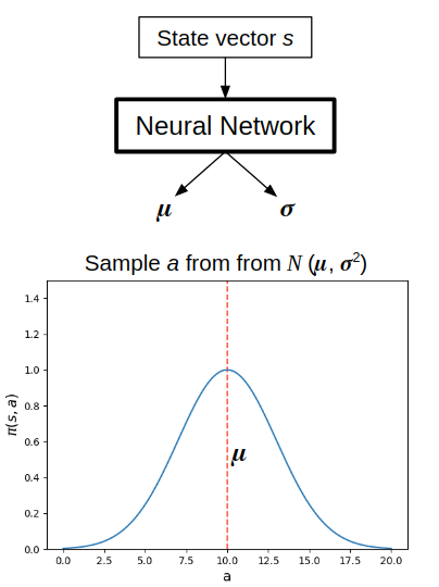
The entropy (more on that below) is similarly calculated; since it's essentially a measure of how much spread the action distribution has (whether for discrete or continuous), here it's just based on $\sigma$. Higher $\sigma$, more spread, higher entropy, more exploration.

That's the way some continuous action space algorithms work, by just parameterizing a distribution which actions get selected from. However, one of the ones I used here is a little different, the Deep Deterministic Policy Gradient (DDPG) algorithm. The main paper was from 2015. It's still an actor-critic algorithm, but optimizes for a different term. Like DQN, it also uses an experience replay buffer, and uses a target NN for both its actor and critic NNs. It updates the target ones with a "soft update" technique where instead of periodically copying the whole thing over, it makes the target update all its weights with 99% its own current weights, and 1% the weights of the learned NN. Like the name suggests, the biggest difference is that actions aren't stochastically selected from a distribution, it's deterministic: a definite number is given. It's really interesting, because in contrast to the classic PG theorem above, the Deterministic PG theorem is:

$$\nabla_\theta J = \mathbb E_\mu[\nabla_\theta Q(s, \mu_\theta(s)]$$

I.e., instead of doing gradient ascent of $J$ by following the gradient of well performing actions scaled by the returns they're responsible for (a handwavy explanation of the regular PG theorem), here it follows only the gradient of $Q$, but with respect to the policy parameters $\theta$. This is actually pretty easy to do with PyTorch due to how it calculates gradients.

Those are the main points of the algorithms I tried out here. I'll mention some of the finer points specific to each of them below when I talk about them.

 

Results

Enough talk! Let's see some results. For all of these, the mouse's step size is a fifth of the circle's radius, so the fastest it can ever get out of the circle is 5 or 6 steps.

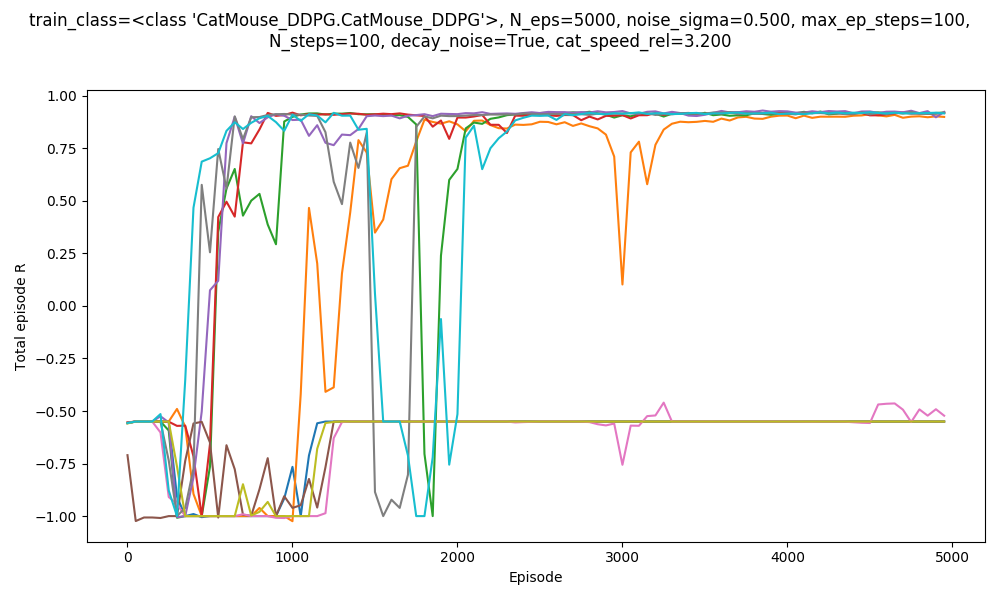
First, using A2C, with $v_{cat} = 3.2$. Here are 5 runs with some mild hyperparameter optimization:

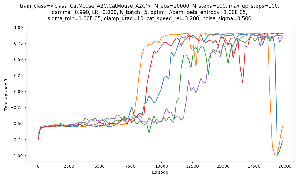
So I could get A2C to work, but it was somewhat finnicky. Further, you can see that the orange and blue runs "crash" at the end. More on that later. Here's mousy escaping at the end of one of the runs above!

However, if we up it to $v_{cat} = 3.3$ (same hyperparameters)...

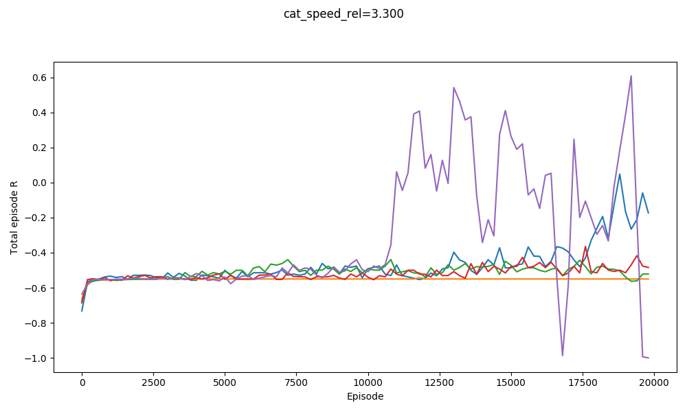
It kind of gets 2 runs, but they're clearly having lots of trouble.

I think a lot of the trouble is with its exploration, which is especially vital in this problem. For a second, pretend there is no cat and the mouse just has to get out of the circle. If it behaves as a random 2D walker (i.e., talking a step randomly in any direction), it will have a mean position of (0, 0) but still randomly get out of the circle eventually. Now consider the easy case with $v_{cat} = 3.0$: it's much harder for a random 2D walker to get out of this, because it requires randomly going in the same (specific) direction several times in a row!

Exploration is encouraged in A2C by adding an entropy penalty term to the total loss, which encourages it to keep the $\sigma$ output of the NN artificially higher. However, this just increases the variance of the normal distribution $\pi (s, a)$. This does increase exploration in the sense of making it take actions it wouldn't otherwise, but not helpfully; it'll just make it more of a random walker. So I suspect that in this problem, when it does get one of its first successes, it's probably when the weights happen to have some random bias that cause it to "always go left" or something, and that will eventually match up with the cat starting on the right.

DDPG is different! Because it's deterministic, it would never explore on its own. So, a common strategy is to explicitly add a noise term to the action output, and then update using that modified action (helpfully, you don't have to deal with importance sampling here, because it's not integrating over actions anyway, which is nice). A common choice is to use Ornstein-Uhlenbeck noise (OU noise), which is basically temporally correlated noise. This is perfect for this problem due to what I was saying above: because each value is related to the previous value, it tends to give rise to "trajectories" more than a random walker's "stumbling", allowing it to escape more easily.

For example, here are 3 Gaussian random walkers with $\sigma = 0.1$, with the actual noise on the left, and their paths (i.e., cumulative sum) on the right:

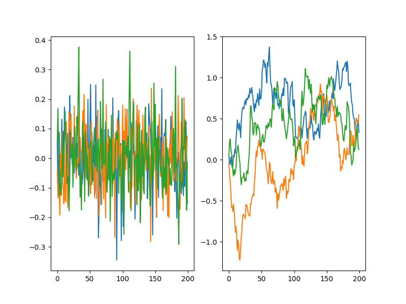
Instead, with OU noise:

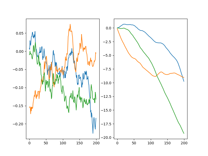
You can see that the OU noise walkers get to a given distance from zero much more quickly. The DDPG paper said they used OU noise, but I've seen a few places mention that it might actually not be more effective than plain ol' Gaussian noise. That's kind of surprising to me. To check this out, I tried DDPG with both Gaussian noise, and OU noise (both with the same $\sigma$) for $v_{cat} = 3.2$.

OU noise:

Plain Gaussian noise:

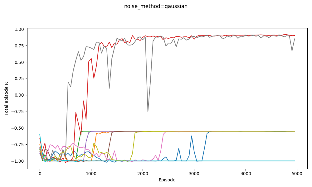
Clearly OU works better. I think one possible cause is that this is a special~~ problem, where having temporally correlated noise/actions is really important for exploration, whereas it's not in many environments. As that link mentions, I also decrease the amount of noise throughout the episode, because after it has explored enough, the noise only hurts performance.

Anyway, I found much more consistent results with DDPG, so everything else I'm showing here is using it rather than A2C.

Recall from the video that the difficulty of the problem is determined by $v_{cat}$, the multiple of the cat's speed compared to the mouse's speed. The value of $v_{cat}$ creates three "regimes": for $v_{cat} < \pi$, the mouse (always starting from the center) can just go in the opposite direction from where the cat starts and always escape. For $v_{cat} \geq 1 + \pi$, there is no solution. In between these extremes, it can use the clever solution, though it only needs to to varying degrees depending on $v_{cat}$; for example, for $v_{cat} = \pi + 0.01$, it barely needs to "curve" away from the cat at all, while for $v_{cat} = \pi + 0.99$, there's only a very narrow margin where it'll work.

So while I wanted to immediately throw it at $v_{cat} = 4.0$, I quickly realized how nearly impossible it would be: at the beginning, everything it does will essentially be random, so it has to discover the solution randomly as well. Can you imagine how difficult it would be to randomly guess the exact sequence of moves that you'd need to escape with $v_{cat} = 4.0$ ? Worse, even if it did that sequence 99% correctly but then got caught at the very end, that would reinforce that it shouldn't do that.

For example, here it is solving $v_{cat} = 3.0, 3.1,$ and $3.2$:

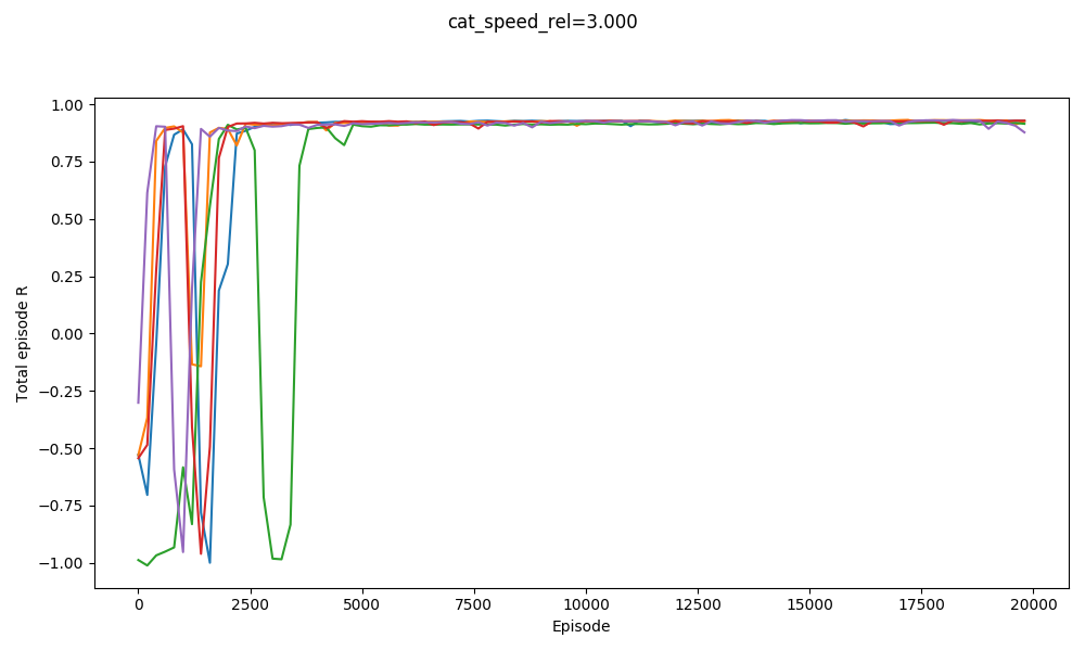
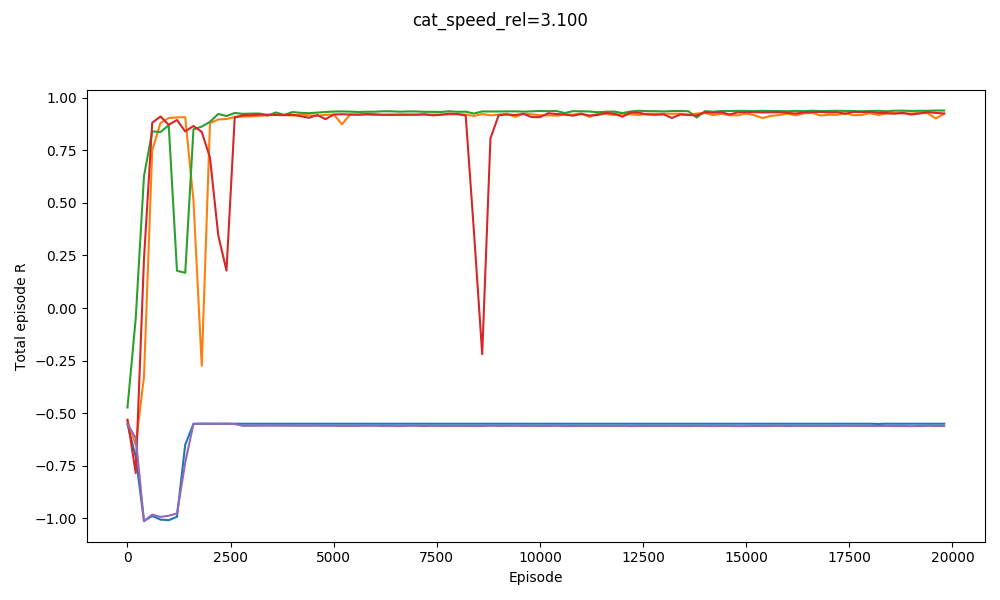
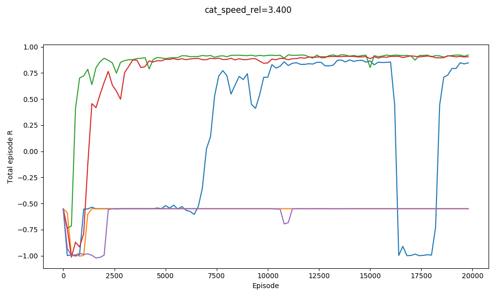
You can see that it basically gets them all. It actually does slightly worse on $v_{cat} = 3.1$ than $v_{cat} = 3.2$. It does badly with $v_{cat} = 3.3$, but manages to get a few with $v_{cat} = 3.4$:

On the other hand, here's jumping straight into $v_{cat} = 3.5$:

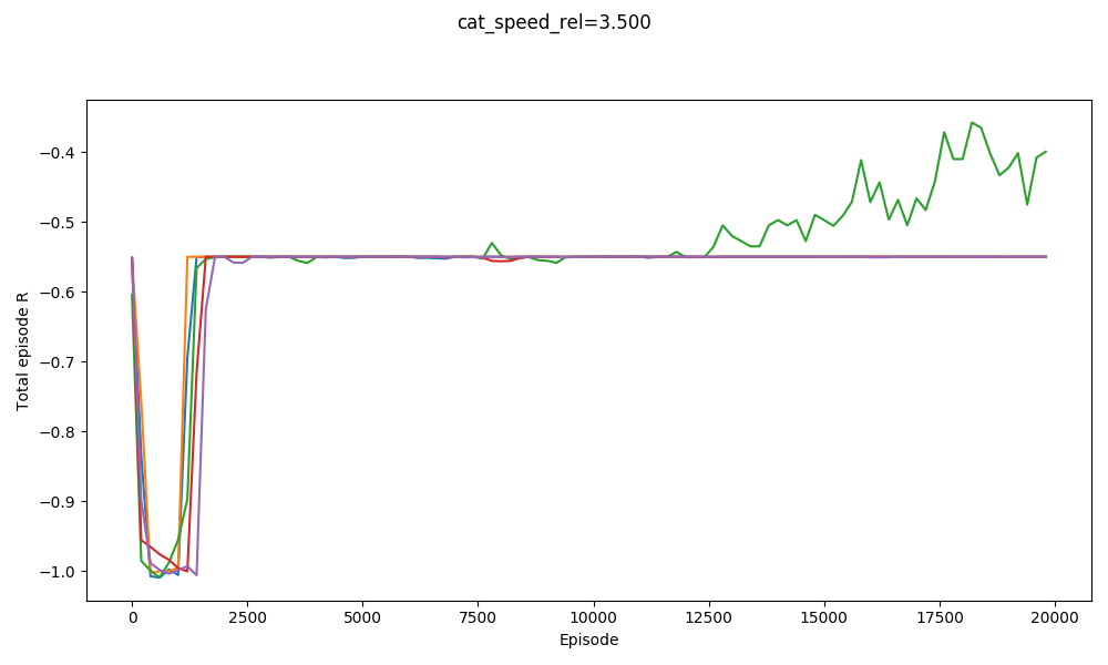
Not so good. It manages to maaaybe get one. It definitely wouldn't be able to start with a $v_{cat}$ any higher though!

So, I "cheated" a little bit, if you want to call it that (though I prefer to call it "incremental bootstrap learning" :P). I realized that when it tries to solve it with a high $v_{cat}$ like 3.5, the main problem is that it's just never given a positive example, because it never escapes once with its random behavior; it can't learn to get to a goal if it doesn't know a goal exists. But, if it learned to beat, say, $v_{cat} = 3.2$, it wouldn't be too much of a stretch for it to then learn $v_{cat} = 3.3$; it would just involve it refining its policy and value functions so they decreased the values of some specific state/action combos that used to be good but now won't work that the cat is faster.

From there, you could obviously "ramp" up the difficulty repeatedly. How does that work? Here it is starting at $v_{cat} = 3.2$, and then increasing to values 3.3, 3.4, 3.5, 3.6:

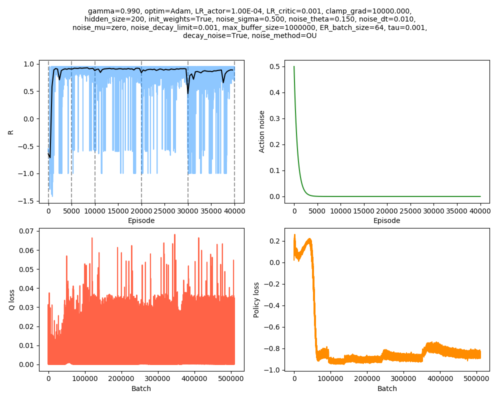
Much better! It was still doing decently at $v_{cat} = 3.6$. It seems like it was happening to get many -1.0 episode scores (meaning it used up all its episode steps and never escaped), but appears to be on an upward trajectory. The black line is a smoothed average of the individual episode scores, and then dashed gray lines show the regions where it has a specific $v_{cat}$, or "epochs" as I'm calling them. Interestingly, you can see a pretty distinct drop at the beginning of each epoch, where the mouse is suddenly being caught in a bunch of circumstances it probably wouldn't have been before. Note that I gave the epochs different numbers of episodes; I suspected that the higher ones would need more time to refine and improve.

I had to do a few interesting little things to account for the fact that doing this made it now a non-stationary environment. For example, DDPG uses an experience replay buffer, where it saves the $(s, a, r, s')$ tuples it previously observed. However, here, the experiences from a previous epoch are invalid! When the cat moves faster that before, the new state $s'$ after doing action $a$ in state $s$ isn't the same as it was before! Therefore, I made it empty the ER buffer at the beginning of each epoch.

I tried a few things to get it higher. Here, I used smaller $v_{cat}$ increments, with $v_{cat} = [3.2, 3.3, 3.4, 3.5, 3.6, 3.65, 3.7, 3.75]$:

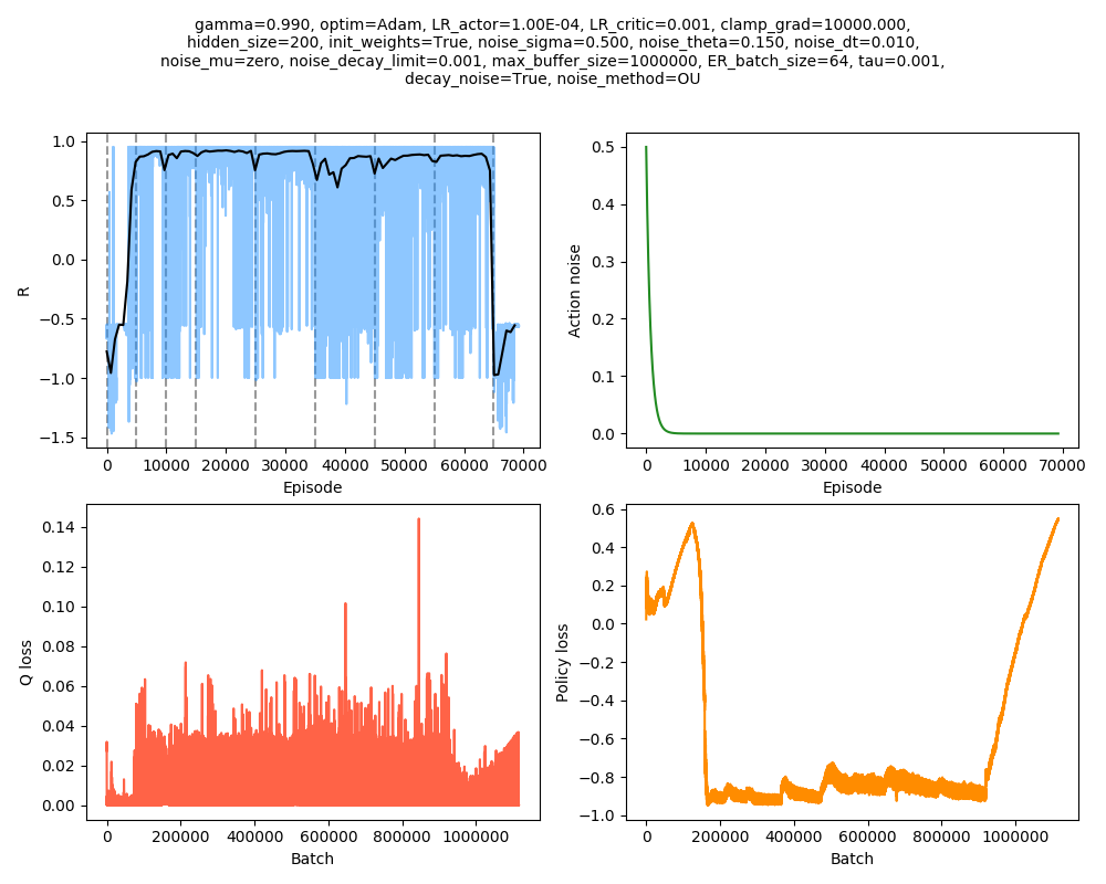
I stopped it in $v_{cat} = 3.75$, because from experience, once it goes down to that level, it's not coming back up! However, it seems like in almost all the epochs, it was actually improving even up until when it switched to the next one. It's pretty cool seeing it escape with $v_{cat} = 3.7$!

What's kind of interesting is that it figured out a weird way to do the trick of going around between the two circles, often inefficiently. I made some fun gifs by saving a model that was trained up to a high $v_{cat}$, and then reloading it and decreasing the mouse step size (and cat step size to match):

Sometimes, it tries multiple passes where it almost gets there, but has learned that it'll have to turn back:

I think its task may be made slightly easier by the fact that it doesn't take infinitesimal steps, it takes relatively large steps, allowing it to cut across the inner circle. It also has the effect you can see in some gifs, where it's able to "switch sides" back and forth quickly at the beginning, making the cat waste time retracing its steps. It couldn't really do this effectively if its step size was smaller. In fact, when I make the step size very small, it can't solve it with $v_{cat} = 3.7$, I have to drop it to about 3.5, and then it still takes some pretty roundabout paths:

I experimented a little with trying to get it even higher, but I didn't make much headway with the few things I tried. Maybe in the future, I'll come back to this and try a few other things that could potentially help:

• Increase the noise at the beginning of epochs
• Reset the optimizers at the beginning of epochs
• Use a smaller ER buffer, and do more frequent, but smaller increments to $v_{cat}$

Till next time!