[latexpage]
Last time I messed around with RL, I solved the classic Mountain Car problem using Q-learning and Experience Replay (ER).
However, it was very basic in a lot of ways:
- There are really only two actions, and the state space had only two dimensions (position and velocity).
- The way I was representing the state space was very simple, "coarse coding", which breaks the continuous state space into discrete chunks, so in a way it still has discrete states. More interesting problems have continuous, many dimensional state spaces.
- The representation of Q was just a state vector times a weight vector, so just linear. You can actually get a decent amount done with linear, but of course all the rage these days is in using neural networks to create the Q function.
- The problem was very "stationary", in the sense that the flag (where the car wanted to go) was always in the same place. Even if I had the flag move around from episode to episode, the strategy would always be the same: try to pick up enough momentum by going back and forth. A more interesting problem is one where the goal moves.
Today, I solve a problem that improves on all of these! And dang, was it a hefty learn for me. I divided it up into sections, so skip around if you don't want to read a bunch.
A classic RL problem I found while watching this David Silver lecture is Puckworld. Here the agent is a little "puck" in a limited 2D plane. It can apply a "thruster" in 4 (U, D, L, R) directions to move (here it can only apply it in one direction at once, but the time step is small enough that it can basically go in any arbitrary direction by switching between thrusters quickly. The same applies to the magnitude; it's set for each thruster, but in between values can be gotten by switching akin to PWM). The goal is for the puck to get close to another little disc, the "target", which is stationary. However, when the puck finds the target, the target moves to a new location. Typically, the state information the puck agent has is a vector of its position, its velocity, and the current position of the target.
To break up the wall of text, here's a little gif I made of one agent after training:
You can see a great interactive demo of it here, on Karpathy's website, I guess from back when he was at Stanford. It's very cool and was pretty helpful for me while doing this. As an aside, while Mountain Car is one of the most characterized RL problems, there's surprisingly little info about Puckworld out there, unless I missed all of it in my Googlin'. So maybe this can help anyone else who tries doing it. Also notice that he adds an enemy that chases the puck and gives it negative reward, which is really cool (maybe I'll add that in the future!).
Reward shaping and reward hacking
One difference though, is that he does his reward function differently. This is actually a pretty big deal in RL, so I'll briefly take about it. In this very famous blog post on RL, the author talks about "reward shaping". The idea is this. The agent learns its behavior via the rewards it gets. You just want it to solve a problem in the best way, so the most straightforward thing to do would be to give it a positive reward for solving the problem (i.e., getting to the target, or getting to the top of the hill in MC) and no (or a small negative, for taking time) reward for not solving it. This is called a "sparse reward". It's good in that it usually really encourages exactly what you want, but also means it might take a long time to find it and therefore learn. Imagine searching a 100 dimensional continuous space for a reward that's in one tiny volume of it: it's basically a random search.
The alternative is "shaped rewards", where it gets intermediate rewards based on the state. For example, Karpathy rewards the agent more based simply on the distance from the target. From was I've seen, there are two main disadvantages to this. The first is that (see the hilarious examples in the above blog post), very often, the agent will "reward hack", meaning that it will do some unexpected behavior, encouraged by the reward shaping you've done, to increase its reward. Usually, it's not really solving the problem you wanted solved, but is actually the best option given the rewards it's receiving. The other disadvantage is that...well, it just doesn't seem super "RL-y". That is, lots of the toy problems we solve with RL are basically trivial if you're willing to just code in the model (or solution to it) yourself, so the point of RL is to figure it out without giving it a model/solution. So, even if you did reward shaping correctly, without unexpected behavior, it just feels like less the point of RL to me.
So in this example it makes the searching way easier. You could basically do a local search of wherever the agent currently is, and go in the direction to maximize the reward. It doesn't have to learn to take the difference between the puck and target positions, because you're basically doing that for it!
Anyway, on to the problem. My initial intention here was to implement it with just the Actor-Critic (AC) model, but I ended up taking a somewhat roundabout path to it. When I first implemented it, it wasn't working, so I backtracked a little and implemented it with a regular ol' DQN. That had its own complications/interesting stuff, so I did a little with that, before going back to implement AC. Since this turned out pretty long, I'll save my AC stuff for another post.
DQN approach
So let's start with the DQN formulation. I should mention that since my network only has 1 hidden layer, I'm not sure it even qualifies for the "D" in DQN, but it's a more common acronym, so I'll use it.
A very basic overview of DQN can be seen in the now famous 2015 Deepmind paper, "Human-level control through deep reinforcement learning". It's actually surprisingly readable and straightforward! (I wish typical physics papers made themselves this accessible.) The main idea is that we approximate the state-action value function, Q, with a neural network, and iteratively improve it to improve our agent's behavior. Here, $Q(s, a)$ can be read as "the value of taking action $a$ in state $s$". So, it itself is not the policy (i.e., what the agent should actually do), but getting the optimal action from an accurate $Q$ is easy, so often, we just solve for Q.
Two details. First, in the Deepmind paper, they have to do a bunch of stuff with convnets, because they're having it learn directly from the screen rather than giving it relevant coordinates of stuff in the game. In my opinion, this is obviously cool, but at the same time it doesn't seem like the novel part. I mean, people in 2015 knew about the power of convnets, so it really just feels like tacking on an extra hurdle for the RL, but not anything really new. So my point is, since I'm generating the environment myself anyway and I'm more interested in learning about RL than CNN's, my agent just gets the coordinates of the target, itself, and its own velocity (a 6-vector, since we're in 2D).
The other detail is that intuitively, you might think that if the function the DQN is approximating is $Q(s, a)$, i.e., a function of two variables, you'd want to have as many inputs as you need to input $s$ and $a$ at the same time (so $6 + 4$) and one output, $Q(s, a)$. I think you can do this, but I guessed that it would make more sense to only have $s$ be the input, and have the values of $Q(s, a)$ be the output for different $a$ values, since $a$ is a discrete 4 options here. And luckily, they mention that they do that in the Deepmind paper! It makes a lot of sense, because we end up taking the argmax of $Q(s, a)$ over $a$ many times.
The other question is about the architecture of the NN. If you take a look at the Deepmind paper, most of their NN is actually the CNN part. Only at the very end do they use fully connected (FC) layers:
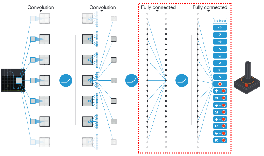
So, there's really only 1 or 2 hidden layers (depending on what exactly they mean), because the first one from the left (in the dotted box I drew) is just the output of the CNN section, so it can kinda be described as the state values, which will be the input layer of our NN. They separate the FC and ReLU parts of the next layer (which is often just considered to be one layer), and then have the output layer.
This is also what I've seen in most DQN papers, so this is what I did (though I experimented with 2 hidden layer ones as well). So, my architecture was an input layer of 6 nodes, a hidden layer of N nodes (I vary this, see below), a nonlinear function (I vary this too), and then an output layer of 4 nodes. Here's what it looks like:
class DQN(nn.Module):

    def __init__(self,D_in,H,D_out,NL_fn=torch.tanh):
        super(DQN, self).__init__()
        self.lin1 = nn.Linear(D_in,H)
        self.lin2 = nn.Linear(H,D_out)
        self.NL_fn = NL_fn

    def forward(self, x):
        x = self.lin1(x)
        x = self.NL_fn(x)
        x = self.lin2(x)
        return(x)
Lastly, as they do, I use Experience Replay (ER), which is actually very important. This means keeping a "target" (or "frozen") network, which is used for part of the error calculation, and periodically updating that network with the "current" network (some people call it the "policy" network). In Torch, this is very simple. You just load the state dict from the current network to the target network:
def updateFrozenQ(self):
    self.target_NN.load_state_dict(self.policy_NN.state_dict())
That basically just copies the weights and biases.
So, how does it do? Let's start with a fun gif of it after learning:
Lawdy, I love watching it zip around like that.
Anyway, since it's most of what I'll be showing, let me briefly talk about the "dashboard" above, which I use to see the behavior of the agent, as it learns. The upper left is the puck agent (red) and target (green). The upper middle is the x and y coordinates of the agent. The upper right is the current reward the agent is getting. You can see that it's mostly -0.01 except when it's at the target, where it gets 1.0. The middle is the x and y velocities. The middle right is the current action that the agent is selecting (the indices are a little messed up in the gif, but typically actions [0, 1, 2, 3] map to [U, D, L, R]). I made all these only show the last 1,000 values, for easier diagnosing.
The bottom left is an approximation of the value function. The color is the value of the agent being at that position; you can see that darker red is closer to the target (more explicitly, since my $Q$ function is a NN, it's evaluating $Q(s)$ for each box, where $s$ is the state vector if the target was in the marked position, the agent was at the location being evaluated, and it had 0 velocity. It then takes the max of the output of $Q(s)$ to get the "best" value). The middle bottom is correspondingly the best action at a given position; it's essentially the argmax of the thing described for the bottom left. When it has learned well, you can see that it's forming a nice general strategy of "if the target is to the R of me, go R". It even forms nice diagonals if the agent is both to the left of and below the target, where it pretty cleanly divides whether it's better to first go right or up in that position. Lastly, the bottom right is the total cumulative reward, which is generally a good clue that the agent is learning, if it increases over time.
Alright! All that said, there are lots of details I learned while doing this, which I'll say a bit about.
DDQN: probably not necessary for this problem
Double DQNs (DDQN) were introduced in yet another Deepmind paper. The idea is that, in the original DQN formulation, the TD target is $R + \gamma \textrm{max}_a Q(s, a, \theta^-)$, where that max of $Q$ over actions $a$ is calculated using the target network (hence the $\theta^-$). Apparently, this tends to overestimate values, and they found that a fix was to split the max up into evaluating the function at the argmax (which would usually be equivalent to the max). However, they instead used the fixed network to get which action is the argmax, and then use the target network to actually evaluate the $Q$ value with this action. So, the TD target ends up being $R + \gamma Q(s, \textrm{argmax}_a Q(s, a, \theta), \theta^-)$.
If I'm honest, I get the idea but still don't have a great intuitive grasp of just why this works. It ends up feeling like the whole "extra frozen target network" thing was a tweak of the TD target to get stability/convergence, and then this DDQN solution is a really similar tweak to the TD target. So maybe I'll think about why this works more thoroughly sometime, because most of the stuff I see using it on the internet just say "it prevents overestimation of the $Q$ values" in a very handwavy way.
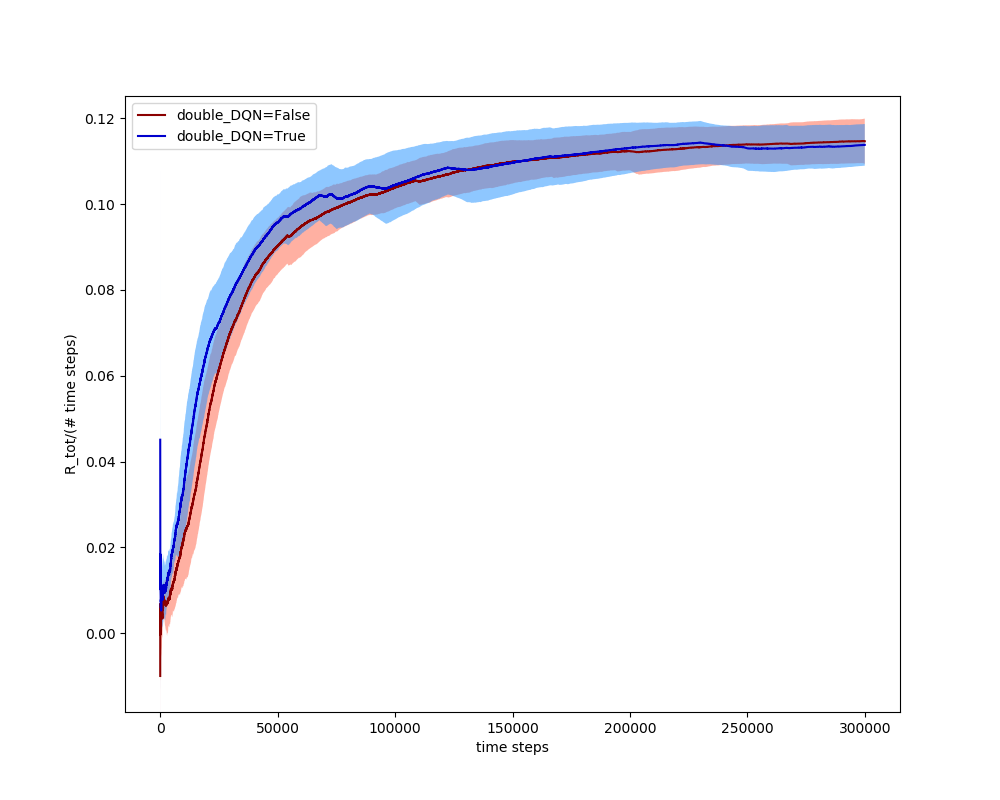
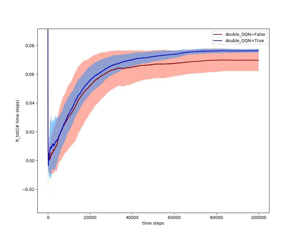
Originally, I was using some minor method (unrelated to DDQN) that turned out to be messing stuff up, and using a DDQN seemed to mitigate the problem more than a vanilla DQN did. However, once I got rid of that, it turns out that DQN and DDQN perform very similarly in Puckworld:
However, I've found that messing around with other parameters shows DDQN to behave slightly better than DQN in general. For example, the best target_update value (how often I update the target network from the current network) I've found is 500, and the best exploration policy is $\epsilon = 0.9, \epsilon_{decay} = 0.9995$, but if I use the very subpar values of target_update = 20 and $\epsilon = 0.9, \epsilon_{decay} = 0.9995$, you can see that they both do worse, but the DDQN trials have a higher mean and way less variance than the DQN:
So, from now on, unless I say otherwise, I'll be using a DDQN.
Varying many parameters and methods: reward shaping, NN nonlinear function, epsilon exploration, loss method, NN hidden layer nodes, target network update, gradient clamping
At this point, I had added a ton of different tweaks to my system in an attempt to fix this problem, so it was easy to test what worked better with the working solution. I also made a nice varyParams() function, where you can give it lists of the parameters you want to scan over, and it runs episodes with them and plots the resulting average rewards at the end.
For each parameter combination, I run several (usually 3-5) runs with those parameters. Obviously, more would be better, but I've learned that in RL it's absolutely vital to at least have a bit of a sense of what kind of spread in behavior the agent will do. Too many times I've ran with some parameters, seen good results, and immediately ran again to find it completely flop. I don't really use them here in a quantitative way, even if more trials would reveal info of that type; I really use them to see if a given strategy is relatively repeatable (i.e., if its variance is low enough that several runs have similar results).
Shaped vs sparse rewards
As I talked about above, shaped vs sparse rewards is a big topic. I was curious about how it would affect the learning rate for the same agent. For the shaped reward here, I just made the reward linearly increase the closer the puck is to the target, so it always wants to get closer to it but there's no special reward for getting to it. Because I'd have to carefully design the scaling factor to make the total average reward equals equal for the shaped and sparse reward methods (which I think would be hard to do without trial and error), here I just shifted the curves after the fact (they didn't need any scaling, though):
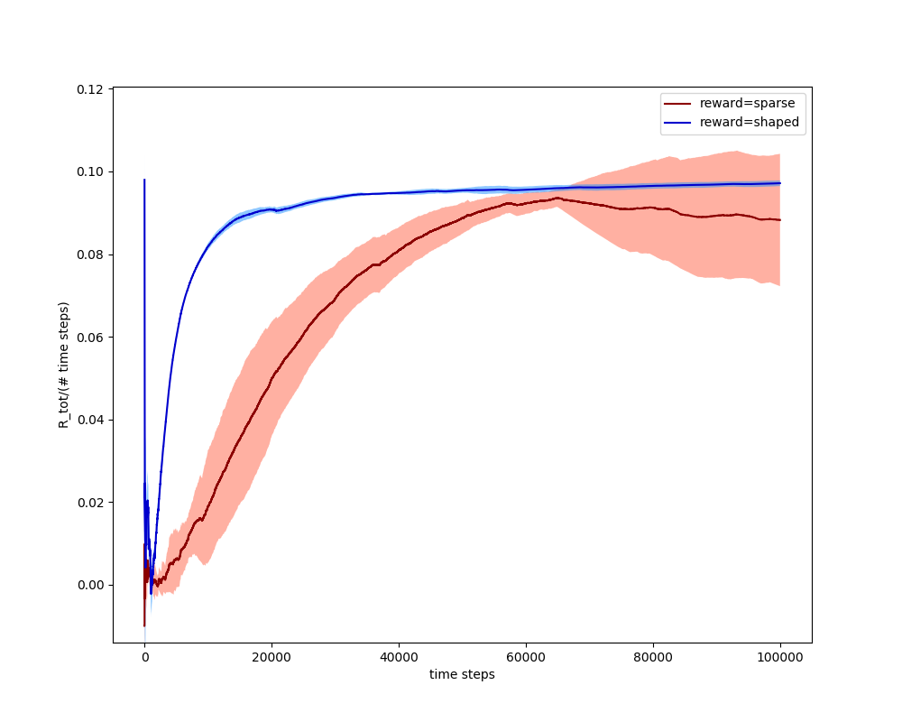
You can see two major things: the shaped reward reaches a large fraction of its equilibrium value wayyy faster, and it has very little variance. This makes sense: for the shaped one, nearly every episode is the same, because it's always getting some reward, no matter where it is. So, you can see that it's a much easier problem, because you built the model more into it.
NN nonlinear function
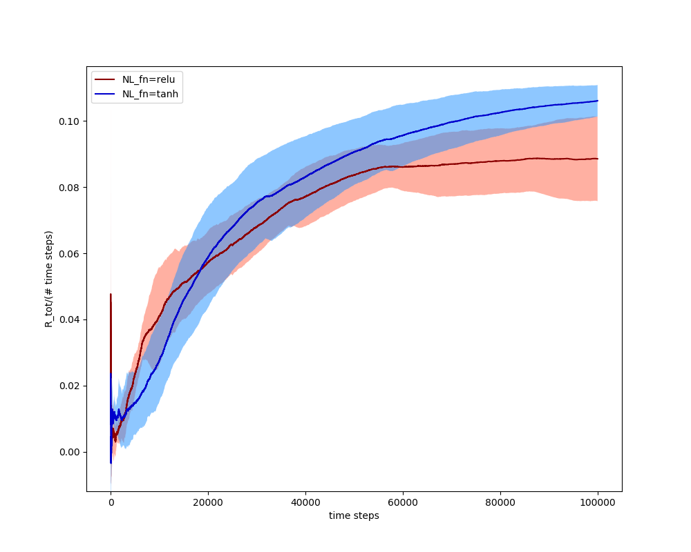
A ReLU seems to be the most common nonlinear function used in NNs these days, but I wanted to try others. While I was flailing around, trying to get my DQN to work, I found that using the tanh function actually seems to give slightly better behavior:
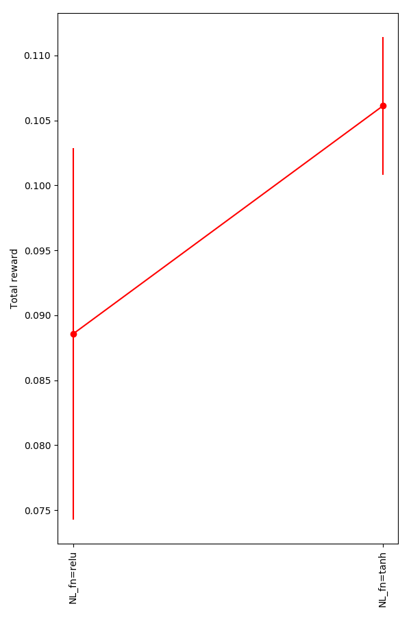
You can see that they're not doing anything crazy, for some reason tanh is just slightly better:
Epsilon exploration
$\epsilon$-greediness means that, some small percent of the time, the agent will take a random action instead of the greedy one. People often either keep a small random element during the whole episode (maybe 5%), or they "anneal" by starting off with $\epsilon$ and "decaying" periodically by multiplying it with some other constant that's less than 1. This will make it decay to 0 over some time period. People also sometimes use an exponential plus a constant term, so they can have it decay to a finite, nonzero value, but I didn't do that here.
I compared three strategies here: greedy, constant small exploration, and large initial epsilon, decaying to 0. Since this was run with $10^5$ steps, for the decaying one, $\epsilon \sim 0.006$ by step $10^4$, for example.
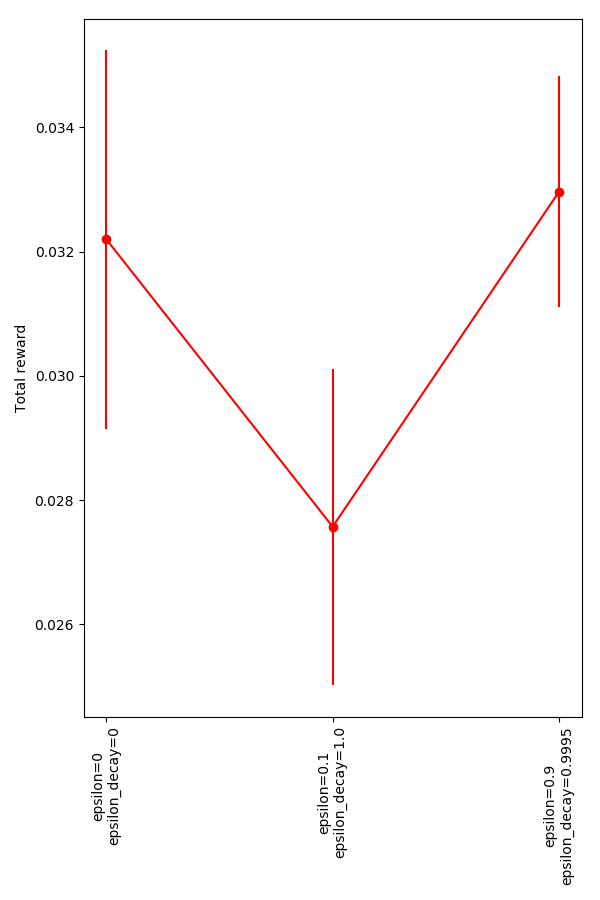
Not a lot of difference, given the variance and the general magnitude of them. It seems like the one thing that might be taken from this is that the "always a little random" strategy isn't great, as you might expect: after a long time, if its has learned correctly, that will just make getting to its target harder, decreasing the total reward.
Loss method
The classic "loss" method to use for stochastic gradient descent with the TD error is minimizing "L2", i.e., $(R + \gamma Q' - Q)^2$ (using some shorthand). This is good, because it punishes very wrong values much more and makes it so the loss is positive, whether the target is bigger than $Q$ or not. However, many people say that it can cause instability, because of the larger gradient due to large losses. Therefore, some people use the "smooth L1 Huber loss". I compared them here.
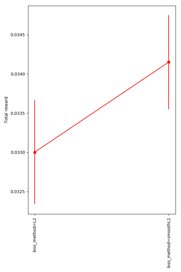
You can see that it does do a bit better, but... barely at all, given the variance.
NN hidden layer nodes
This one was interesting. I use a NN with one hidden layer for all of these, but I didn't have a great concept of how many hidden layer nodes (HLN) would be needed to learn the strategy. It seems like the main thing it has to do is evaluate the position of the agent ($p$) and target ($t$), and then just send it in the direction dictated by the sign of one minus the other. That is, if $t_x > p_x$, then the target is to the right of the agent, and the agent has to go right, and give a high number to the output node corresponding to R. It might seem like it would also have to have some sort of "comparator" when the target is, say, both to the right and above the agent, and it needs to decide which action is more pressing, but that's really done by the argmax: the outputs for U and R would both go high, but the more important one would go higher, and the argmax would choose them.
So, if I had to guess, the NN could probably even do it with 2 HLN! The connections from the hidden layer to the output nodes let one HLN determine the L and R outputs (opposite signed weights), and the other node can handle U and D (same idea).
So I knew that it could probably be done with a reaaally simple NN, but here are the results:
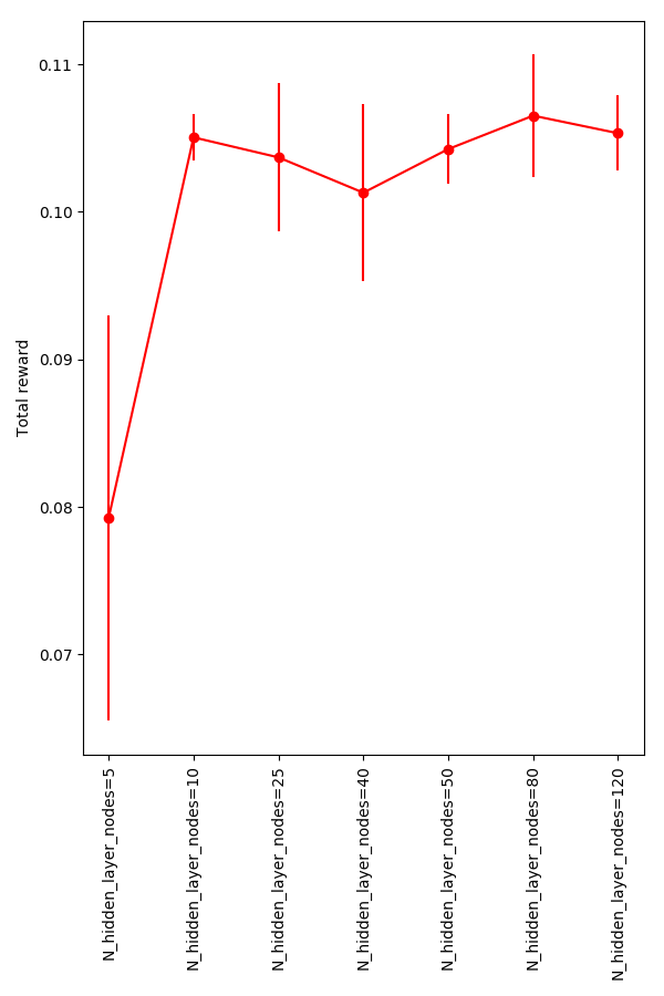
So the performance definitely goes down for 5 HLN, but it seems like the others are roughly equivalent. I wanted to see where it "breaks", so I looked at the smallest range and a large range:
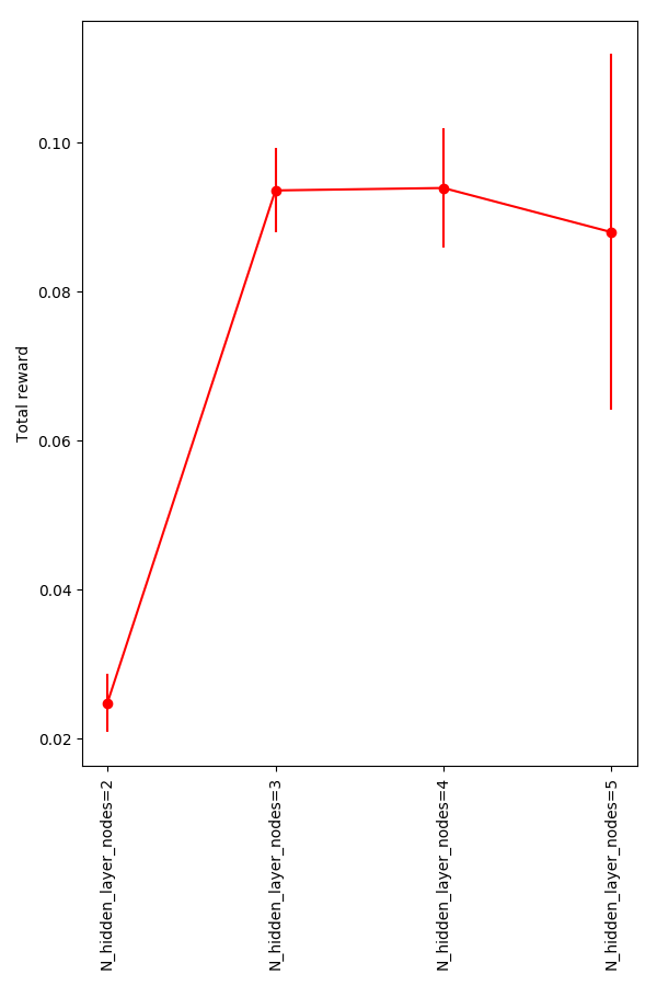
Definitely significantly degraded for 2 HLN.
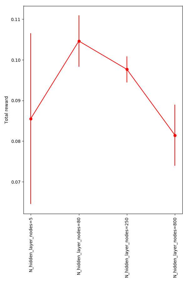
And, it seems like 800 HLN is too many.
Interestingly, if we look at the plot of the average over these runs for the 2-5 HLN one, we see that the 2 HLN set still learns, but it never gets as high as the others:
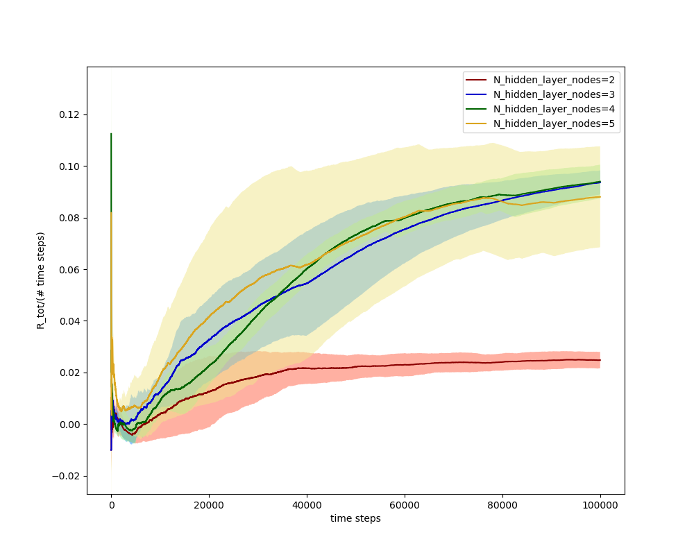
So it seems like there's a significant gain in having that 3rd HLN. I wonder what it's adding? This might be worth looking into at some point.
It's possible that it could actually use the velocity info cleverly (i.e., if it were currently going in the opposite x direction from the target, but had figured out it could retain speed and get there faster by bouncing off the wall), which might need more nodes/layers, but I didn't see any evidence of that.
The 800 HLN one doesn't do notably worse than the others, just slightly. They're also all still improving, as you can see, so it's possible we'd see different results if I let it run 10x longer.
Target network update
This is one that is both a significant effect, and I'm also unclear about. As mentioned above, with ER or DDQN, you have to periodically update your target network with the values of the current network, or you'll be using old information. But how often should you update?
The two opposing effects here are 1) if it goes too long between updates, you'll be using older Q values to calculate the loss, and 2) if it's too often, the networks won't be different enough, and the network won't be stable, but it's not clear to me where the sweet spot is. However, there does seem to be one:
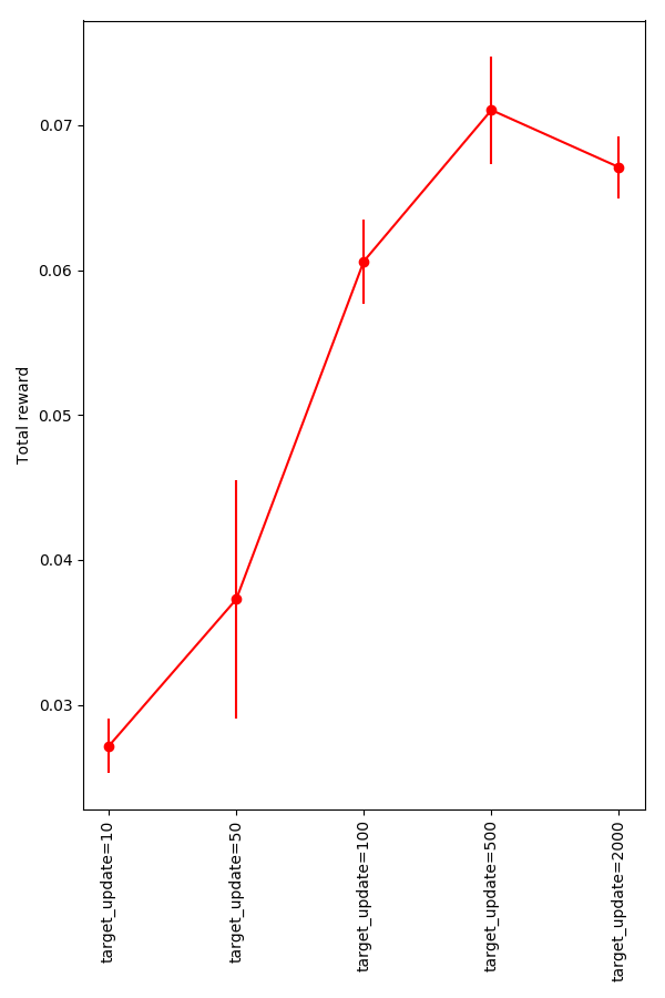
The difference between these average rewards is definitely meaningful, and their variances are generally reasonable. It seems like in the ballpark of 500 is best.
Other notes
Here are a few other things I learned from this project.
GPUs aren't super useful here
I thought that this time I might try to get some AWS time and speed up my runs, but I hadn't thought much about exactly how that would help. It turns out it doesn't, here. GPU use really shines when there's a ton of parallel computation to do, so they're great for training/running NNs on huge datasets, like in many deep learning applications. However, they seem to not be as useful here, because there aren't any places where I'm doing huge batches of stuff with the NN. Even though I'm doing the ER thing, it's still not that huge, and I don't think big enough to justify using a GPU (which involves a bunch of overhead too). I tried it a bit and found that to be the case.
A generalized Agent class
This is more just a thing for myself, but I wanted to make a more general Agent class, so I wouldn't have to repeat the same stuff again and again for different environments. So the actual structure of this program is such that there's an Agent class, and then a PuckworldAgent class too. You pass the class of the specific agent (PuckworldAgent, for example) to the Agent constructor, and then it does everything from there. The specific agent is responsible for having a few named functions that the Agent class will call, like reward(), getStateVec(), and iterate(), but otherwise, the Agent class doesn't know anything about the specific agent class, so it's very general.
The specific agent is also responsible for its own graphics; for example, in the images above, the top left image of the current state is drawn by the specific agent class. Agent has its specific agent object call a drawState() function, which it passes an axis for it to use. This will be nice for comparing different custom environments quickly if I ever want to, also.
The physics of it
In my mountain car post, I talked a bit about how the physics could be important, because you don't want it automatically gaining energy, when that's the goal. Here, that's not so important, so I used a plain ol' Euler-Cromer integration. I'm sure there are lots of ways to do this, but for the environment, I gave it a decent amount of drag, which will slow it down and prevent it from going to fast. It also has an "acceleration" term that determines the impulse when it chooses an action.
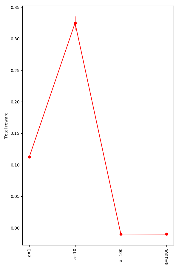
One thing I wondered about is, if you made the acceleration too high (and the drag not able to cancel it out), would it be able to learn? It seems like if it was basically uncontrollable, it shouldn't be able to. On the other hand, if there was no drag and it could speed up infinitely, and it still bounces off the walls bounce elastically, a great strategy could be to gain as much speed as possible, and bounce at a slight angle from the horizontal. This would make it essentially "scan" the whole space, and be sure to hit any target much more quickly than if it had to stop and change direction each time. Does it?
From $a = [0.1 - 10]$, you can see that having a higher $a$ basically just lets it get there faster, so it works better:
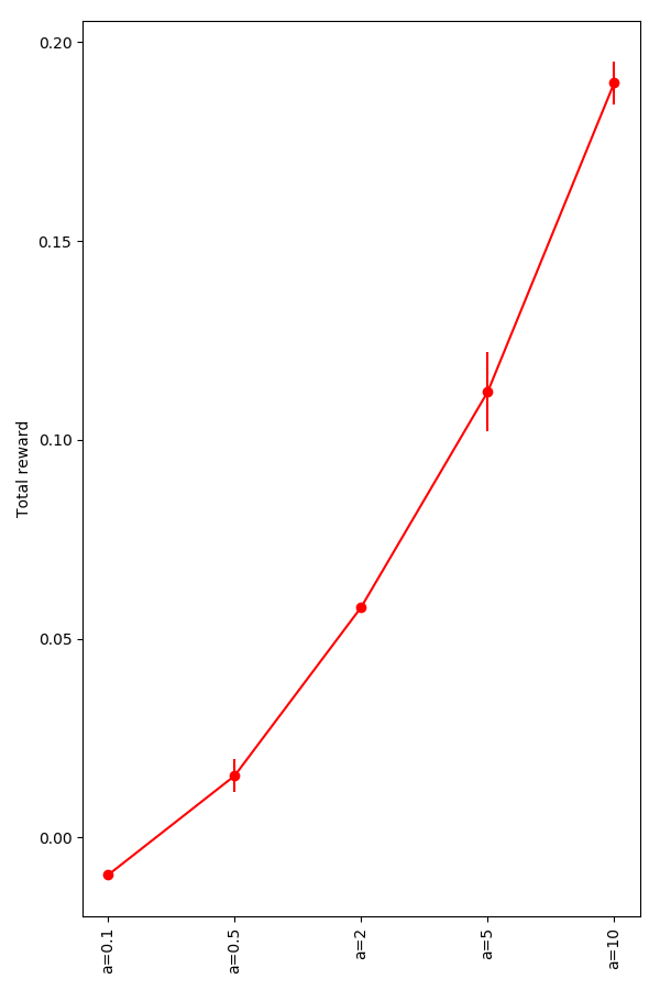
However, for 100 and up, it apparently doesn't learn this "advanced" strategy:
That's all for now. Later!