[latexpage]
In my first post on Genetic Algorithms (GA), I mentioned at the end that I wanted to try doing some other applications of them, rather than just the N Queens Problem. In the next post, I built the "generic" GA algorithm structure, so it should be easy to test with other "species", but didn't end up using it for any applications.
I thought I'd do a bunch of applications, but the first one actually ended up being pretty interesting, so... here we are.
The code used for this is here. It's a little opaque, so message me for any questions or feedback.
The brachistochrone problem
This is a very old, very famous physics problem. It goes like this. Let's say you have two points, A and B, where A is some lateral distance away from B, and some height above B. You have to attach a rigid wire between these two points, in any shape you want, such that a bead sliding down the wire due to gravity, will take the shortest time possible. "Brachistochrone" is Spanish or Japanese or something for "shortest time".
For a first guess you might just imagine using a straight line between them, but that's actually not the fastest route! What is the fastest route is a problem that took some of the greatest minds like Newton and the Bernoulli brothers to solve. To cut to the chase, here's an animation from Wikipedia of the fastest route and two other slower ones:
It turns out that the fastest route is a section of a curve called a cycloid, that is formed by a point on a circle tracing out a path, as the circle rolls along a line:

An intuitive explanation for why you might expect some weird shape (as opposed to the two worse ones in the gif above) is that the any curve for this problem is a tradeoff between two things, speed gained and distance traveled. Speed is gained from dropping vertical distance, converting potential energy to kinetic.
Gaining speed is really necessary for the bead, because gained speed makes the rest of the path take a lot less time. For example, look at the path in the first gif that has that sharp right angle: it gains literally all the speed it can immediately (by dropping vertically), and then travels at a constant, fast rate across its whole horizontal section. The actual ideal solution actually doesn't beat it by a whole lot. Comparing it with the line segment that goes straight from A to B, you can see that that one spends too long gaining speed, and is the worst.
Of course, the other side of this balance is that while the right angle path above gains speed very quickly, it covers no horizontal distance while it's doing that. So it gets beaten by the brachistochrone solution curve, which reaches the same vertical height a little later but has already traveled some horizontal distance, which makes all the difference.
Anyway, I thought this might be a fun application for genetic algorithms (GA). My strategy is pretty simple: a candidate solution ("individual") path will be a list of (x, y) points from the starting to ending point, connected by straight line segments. The fitness function (FF) will be the time it would take a bead to fall down that path.
So, here's an example of a (very bad) candidate solution in black, with the ideal solution in gray:
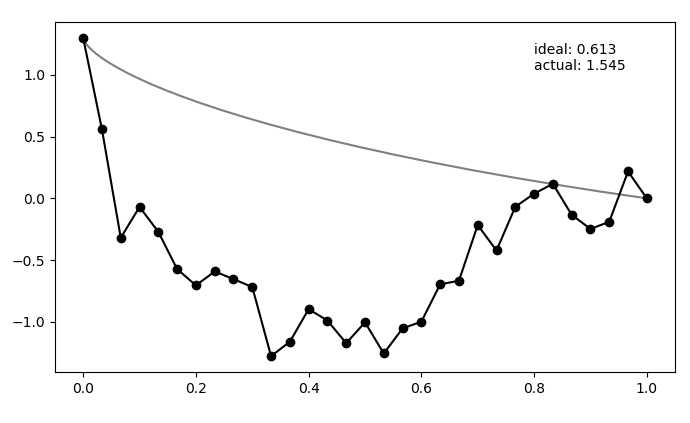 Here, $N_{pts} = 30$, which you can see on the candidate solution.
Mutating is randomly choosing between 1 and N points (besides the start and end points), and changing each from its current position by some amount (more on this below). Mating is taking two candidate solutions and choosing a random set of their corresponding points, and switching them. I (for no real reason) do something here that's actually a little unusual from stuff I've seen in the literature: to mate them, I basically do a Cartesian product of the current population to get mate pairs, mate them, then mutate these, as well as the (unmated) current population, and then take the best of all these and the original population. That involves taking the FF of each, which is usually a way too expensive operation. Maybe I'll change this in a bit, since it's probably very inefficient.
Anyway! So how does it do?
Here it is for $N_{pop}$ (population size) 12, $N_{pts} = 12$, a height of 1.3, and 150 generations:
 Neat! In the top panel, it's plotting the best FF of the population, as well as the mean of the population, which are pretty similar pretty quickly. In the bottom panel, it's showing the whole population at each step, color coded from best to worse (black being the best solution, red to blue going from best to worst). The 'ideal' label is the time needed for the calculated ideal solution, and the 'actual' label is for the best candidate solution.
Let's also try a configuration that has to go below the finishing point, by setting the height to 0.3 instead:
 Neato!
So let's try and vary a couple other things. First, let's add some points. You can see that, in the 2nd example, even after settling, it's still not exactly at the ideal solution. However, that's because the ideal solution isn't limited by the resolution of these points. So, the one it finds might actually be roughly the ideal solution, if you could only use 12 points (...or it could still be a slightly crappy solution).
Here's $N_{pop} = 12$, $N_{pts} = 30$, height = 1.3 again, and for 250 gens:
Hmmmm..! You can see that it actually doesn't converge to the ideal solution, even though the points seem to be converging to something. Doubling $N_{pop}$ (to maybe account for the increased number of points?) doesn't help a whole lot either. Even if I let it go a bunch longer, it doesn't improve much.
Here's where I had a fun little learn!
An important insight for this problem is that, if the current best candidate solution is somewhat far off from the ideal solution but also smooth (like the ending states of the ones above), if you mutate only a single point to the actual solution coordinate, the solution almost certainly wouldn't be chosen for the next gen. Because it would now cause a jagged bump, the bead would have to waste time going up it, which would be worse than the current sub-par solution that's at least smooth.
I think that's the explanation for the behavior in the last gif. A decent solution is found at the beginning when the individuals are chaotic and mostly pretty bad. When mating and mutating happens, the offspring/mutations of this individual are still the best, so the population quickly becomes more like it. However, then it becomes pretty hard for them to get out of that local minimum because of the "disrupting a smooth curve" effect I mentioned above.
I considered that it might be something having to do with how much I mutate an individual, so I experimented with that a bit. When a point to mutate is selected, I add to its y coordinate a random sample from a Gaussian, scaled by some fraction of the total height of the problem, in either the positive and negative direction. So, maybe it either wasn't large enough to find better solutions, or it was too big, and thus, most mutations were way too "jagged" to improve? I don't think the former makes any sense, and the latter might be true, but would ultimately mean taking a ton more timesteps.
No, the problem is something else. It's tempting to say that it's stuck in a local minima, but I don't think this is actually the case (see below).
The fix I came up with was to enforce diversity among the population. I think there are actually several ways to fix the problem (for example, maybe probabilistically accepting individuals with worse FF's), but this worked too.
I did it like so. I actually already had a deleteDuplicates() function from when I was doing the N Queens Problem, since a decent number of the solutions would be duplicates of another. This was pretty easy with the NQP because it's a short discrete list to check, but here I compare two solutions by taking the sum of their differences at each point, and then checking if that sum is under some threshold. If it is, I say they're the same and throw the worse one away (see below for details).
So, to enforce more diversity, you just need to increase that threshold, same_thresh. This will make the isSameState() function reply "True" more liberally, and make deleteDuplicates() get rid of solutions that are too similar to the best one, leaving worse, but more diverse individuals in the population.
So how does it do? Here it is with same_thresh = 0.05:
 So you can see that it's definitely achieving a better solution by the end that the previous one that didn't enforce diversity. However, there are two things to watch out for here.
First, if you look closely you can see the red curves disappearing as it goes on. This is because at some point, too many of the solutions are returning True from isSameState(), and the enforced diversity is actually making the population size go down. Sometimes it will bounce back, after a few lucky mutations/matings, but often it effectively kills it. This also makes the mutation_strength parameter very important, because it will determine how different states can mutate from each other. So you have to scale the mutation amount by the diversity you're enforcing.
Here's an example where the mutation strength is too weak to provide different enough individuals:
However, this is a pretty delicate balance too, because just increasing the mutation_strength along with the diversity will just make it so most solutions are pretty bad, even if the population doesn't collapse. Here's an example with a high diversity, but also a high mutation_strength:
 The states are changing and the population isn't collapsing, but the solution isn't really getting anywhere either.
The other hurdle is that even if you tuned that combo somewhat well, there's a good chance that as it gets close to the solution, it will be really difficult for it to converge nicely, because you'll effectively be allowing only one individual too close to the solution.
At this point I began to see some parallels to a few other search and optimization methods. For example, in simulated annealing (SA), you accept worse solutions than your current one, with some probability based on a "temperature" parameter T. This is good early in the search, because it might lead to a better state that it wouldn't see if it only greedily took states that are immediately better.
This feels somewhat analogous to this diversifying, where I'm necessarily taking worse states because they might lead to something better in the future.
Taking the SA analogy further, if you never decreased T, you would never converge to a good solution, so you "anneal" it over time to eventually let it settle. Similarly, we have to do that here with the diversity requirement, for the stuff I talked about before. To do this, every generation, I multiply that same_thresh by a decay factor. I calculate the decay factor so it will bring same_thresh to about 0 by the end of the evolution,
$decay = (10^{-5})^{\frac{1}{N_{gen}}}$
Similarly, in gradient descent, you usually have to decrease your step size as you get closer to the solution, or it won't converge as well (or even diverge!).
How does it do?
Hot damn! Not bad.
This is pretty nice, because it "scans" the diversity requirement through a range, and at some point in the range, it naturally "matches" the mutation strength in a beneficial way.
However, it's not foolproof -- if the mutation strength is too high, it will screw it at the end, and if it's too small, it will screw it at the beginning, where it needs large mutations to stay diverse.
Here's one more, for the "drooping" brachistochrone:
You can see something pretty cool if you look carefully at the colors of the population. I set it so the colors vary from best to worst, from blue to red, but it's really just a list of those colors, of length (max population size). So, when the population is smaller right after the beginning because of that enforced diversity, you mostly just see the blues. Then the reds come in, as it's allowed to be less diverse and the population grows. Here's the population size over time for that one:
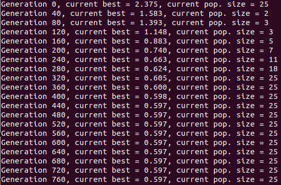
This point where the population picks back up again is actually where it makes a relatively (for being so "late" in the evolution) large amount of progress, such that you can often see a noticeable shoulder in the FF curves, like here around generation 375:
 Anyway, that's it for the fun stuff! This was longer than I expected, so I'll actually do the other stuff in another post, like other applications and comparisons to other search methods. Below is just a little more rambling about this stuff.
I do feel obligated to mention that GA actually probably isn't the best search method for this application, though: the merits of GA for anything (compared to other search/optimization methods, that is) are a contentious issue, but this problem almost certainly isn't a good application for it.
From my brief poking around, it seems like there may not be local minima to this problem. A local minimum is where there's no direction in your N-dimensional space that you could go, that would let you go further down; you have to go up at least a little to get to a lower spot (if there is one). This is just speculation/theorizing based on what I've seen while doing this, but I don't think you actually ever end up in a minimum! (with my setup, anyway.) It seems like the tricky part is that the direction that lets you go lower (in FF) is often a very specific direction. That is, our N-dim space here is the space of all the possible positions of the N points we specify. Like I mentioned previously, it doesn't work to just move one point to its ideal solution location. In fact, it seems like the direction (in N space) you can move to do better in a certain position are a tiny subset of the directions you can take; it's not just which ones have to be moved, but also how much.
Anyway, I mention all that partly because it's what makes this problem kind of tricky for some search methods, and partly because this type of this isn't really what GA excels at (if it excels at anything, heh). If you are in a landscape with no local optima, only a global one, something like gradient descent is probably pretty reliable.
A few details: I actually specify $N_{pts}$ and divide the x (lateral) distance (which will always be 1.0) into that many points. So that could be unconstrained too, but I chose to specify the x points, and have the solution be the y coordinate for each one of them. I also constrain the first and last points to the two points that define the brachistochrone solution.
Because my candidate solutions certainly contain sharp bends, the assumption (to be physical and conserve energy) is that when the bead encounters a sharp bend between two segments, it keeps the same exact magnitude velocity, but now in the direction of the next line segment.
Lastly, if one of the (moveable) points went above the starting point, that would mean it could never get to the end (because the bead wouldn't have enough energy to get over it), I just don't allow any points to go above that first point. I could let them, and make the FF infinity or something, but eh.
I made a little fix to the thing with populations "dying out" when forcing too much diversity. Now, I only do the deleteDupes() thing if the population size (after mating/mutating) is bigger than we need. This actually fixes it pretty much completely, and lets me be pretty cavalier with the initial same_thresh. You can often see the population go low for a while, but then pick up again and solve it.