I've been doing this Coursera Discrete Optimization course with my friends. It's a lot of fun and I'm learning a bunch. The instructor is a total goofball too, which is a plus. I've taken a handful of online courses before, but to be honest, the assignments have usually been pretty easy. Not so with this Discrete Optimization (DO (my initials!)) course! Each week, you have to solve 6 problems, and each is graded out of 10 depending on how well you do. I believe the breakdown is: 0/10 if your answer doesn't even match the output format required, 3/10 if you do basically anything (even if your answer is quite wrong), 7/10 if you have an answer above some threshold but still not perfect, and 10/10 if your answer is optimal (I guess they know the optimal solution for all of them?). Usually, the problems increase in hardness throughout the set; often, the last one is difficult enough that (I believe we saw this said in the course forums by the instructor) it would be a challenge for people who specialize in DO for a living. I think that's pretty cool! They usually give you a ton of practice problems of various difficulties, and (though I'm not 100% sure) I think the 6 you're graded on are usually among those.
So what is DO? I certainly didn't know when I started this course, though I guess I should've been able to guess. Optimization is what it sounds like, finding the best solution you can for given problems. The "discrete" part is that the quantities involved are integers or discrete (that's the name in the title!!!) components. It turns out I had actually heard of many of the problems that DO applies to before, but didn't know they were DO. I had heard most of them in the context of P vs NP complexity.
Anyway, enough of that. Week 1 didn't have an assignment, so the first one was in week 2, and it was the famous "knapsack problem". I'm guessing if you're reading this (sike, no one reads this!), you're familiar with it, but in case you aren't, it's as follows. You have a knapsack with a certain (weight) capacity, K. There are a bunch of items in front of you, and each one has a certain weight (w) and value (v). You wanna fill your backpack with the most valuable (i.e., largest combined value) set of items you can, and you can only take the items whole (i.e., you can't break one in half to fill the bag completely).
Because I'll be referring to it a few times, the format of a given problem (just a text file) they give you looks like this:
n K
v_0 w_0
v_1 w_1
...
v_n-1 w_n-1
n is the number of items there are, and K is the capacity of your bag in this problem. v and w are the value and weight of each item. (I'll refer to the items by their line number, starting with 0, in the following.)
Here's where the "discrete-iness" comes into play. If you were allowed to take non-whole pieces of the items, the solution would be trivial: you would calculate the density (d = v/w) of each item, and start taking the most (densely) valuable items in decreasing order. When you get to the point where your bag can't take the next whole item, you take as much of it as you can fit, and this is the theoretically most valuable set.
Now, for the actual problem (where you can't take fractional pieces of items) it turns out that this is still often a decent solution, for intuitive reasons; denser items are giving you more bang for your buck. This is called the "greedy solution", because it just greedily takes the best item it can at any moment. However, the problem gets interesting when that strategy will actually give you sub-optimal results. In fact, helpfully, the simplest problem they give you already has a non-greedy optimal solution (OS):
4 11
8 4
10 5
15 8
4 3
The items already happen to be ordered by decreasing density. If you did the greedy solution and took item 0 (8, 4) and then item 1 (10, 5), you couldn't take any more items and your total value would be 18. However, this isn't OS! You can see that you actually wanna take the least two densest items, 2 and 3, which perfectly fill the bag and also add up to 19, the OS.
So, that's the problem! Now, how do you actually solve it? (And, what does it mean to solve it?)
The most naive way you can imagine is to try every possible set, and take the largest valid (i.e., all the items fit in the bag) solution. You have a list of n items, so for each one, you can either take it (1) or leave it (0). So there are really only (hah!) 2^n possible sets of items. Naturally, this lends itself to a tree data structure, but it should also be clear that 2^n quickly becomes infeasible for surprisingly low values of n.
Therefore, the real game is in traversing that tree in some clever way such that you don't have to go through the whole tree. I should make a distinction here. There are two types of solution you can solve for. You can go for the OS, where you're 100% sure the solution you end up with is optimal. This actually doesn't necessitate going through the whole tree. Sometimes you can know that you don't need to go farther down a tree, which allows you to not have to look at the solutions contained within that part of the tree, but still know that a solution you find will be the OS. On the other hand, sometimes this is still infeasible, so you have to go for an approximate solution (AS), where you're just doing the best you can. However, not requiring the solution you get to be the OS can let you find great solutions way faster, and still sometimes even let you find the OS. The downside is that you won't know 100% that you got the OS.
So let's actually start. The way my friends and I originally did it (and I stuck with), we actually don't explicitly have a tree data structure; however, by dint of doing recursion with two possible recursive calls, this implicitly forms a tree.
The first thing done is reading in the data and storing it in a list of namedtuple Item objects, which I believe was given to us. Then, because we're going to go through the tree in order of decreasing density, we sort the list by that:
def sortListDensity(inList):
    return(sorted(inList, key=lambda item:-item.density))

lines = input_data.split('\n')

firstLine = lines[0].split()
item_count = int(firstLine[0])
capacity = int(firstLine[1])

items = []

for i in range(1, item_count+1):
    line = lines[i]
    parts = line.split()
    items.append(Item(i-1, int(parts[0]), int(parts[1]),float(parts[0])/float(parts[1])))

sortedList = sortListDensity(items)
We need the function fullItemsStartingValue(), which finds the greedy solution. We'll want this because we're going to judge all solutions we find against the best (valid) one we've found yet, and this is a good starting point.
def fullItemsStartingValue(sortedList,cap):
    #This finds the greedy solution when the list is sorted by density.
    bestEst = 0
    bestEstList = []
    #find first item that actually fits in the sack
    firstItemIndex = 0
    for i,item in enumerate(sortedList):
        if item.weight <= cap:
            firstItemIndex = i
            break
    print("first item that actually fits is index {} with weight {}".format(firstItemIndex,sortedList[firstItemIndex].weight))
    for item in sortedList[firstItemIndex:]:
        if item.weight <= cap:
            bestEst += item.value
            bestEstList += [item]
            cap -= item.weight
        else:
            return(bestEst)
    return(bestEst)
We get this value and set bestVal to it, which I've chosen to be a global:
possibleStartingVal = fullItemsStartingValue(sortedList,capacity)

global bestVal
bestVal = possibleStartingVal
Now, let's dive into our first, most naive implementation. To start, I'm doing a depth-first search (DFS), which means that the tree searches by going as far down into the tree as it can, before trying other branches. I can't actually think of how you wouldn't do DFS here, since you need to go down to the child nodes of a tree to actually get a solution. Here's the most basic DFS implementation we can do:
def solveKnapsackDFS(itemList,itemIndex,roomLeft,valueAccum,acceptedItemIndexList):
    global bestVal
    global bestSet

    #If the value achieved by reaching this node is better than the best value found so far, update the best value and best set.
    if valueAccum > bestVal:
        bestVal = valueAccum
        bestSet = acceptedItemIndexList

    #If we've gone through all decisions and are at the end of the tree.
    if itemIndex == (len(itemList)):
        return(valueAccum)

    acceptVal = -1
    #Try to accept item
    if roomLeft-itemList[itemIndex].weight >= 0:
        newAcceptedItemIndexList = acceptedItemIndexList + [itemIndex]
        acceptVal = solveKnapsackDFS(itemList,itemIndex + 1, roomLeft-itemList[itemIndex].weight,valueAccum+itemList[itemIndex].value,newAcceptedItemIndexList)

    #Reject item
    rejectVal = solveKnapsackDFS(itemList,itemIndex + 1, roomLeft,valueAccum,acceptedItemIndexList)
    return(max(acceptVal,rejectVal))
Here's the basic idea: for each item, you can take it, or not. I first call the function like this:
solveKnapsackDFS(sortedList,0,capacity,0,[])
This is calling the function with itemIndex = 0 (so the first in the sorted list), the entire capacity remaining, no value accumulated (because we haven't added anything yet), and an empty list of accepted items (same). Within the function, we'll make "decisions" that call the function again, but with different arguments reflecting the "decision" that was made. Briefly, for a given call to this function (i.e., we've considered m items already, we're going to call the function again to calculate the values found from accepting and rejecting the next item, and take the maximum of the result of those two function calls. This recursion continues until either we've considered all items, or an item doesn't fit in the bag.
The two global lines are there to access the global best set and value we've found, since we'll want that info no matter where in the search we are. Next, we check to see if, for the current call to this function, its accumulated value is our best yet, and if it is, update that. Then, if the item index of the call is the end of the list, we know we've considered all the items, so we just return what we've accumulated so far.
Then we set acceptVal = -1. -1 is the return value we use to indicate to the calling function that this branch doesn't provide a feasible solution. So, we set acceptVal = -1, and then test to see if the bag has room to accept the next item in the list. If it can, it will recurse again and set that result to acceptVal (which could still end up being -1). However, if it can't, we want acceptVal to stay -1 so it doesn't affect the result of rejectVal, if that provides a solution.
Then we do similar and recurse, but for rejecting the next item. Note that for calling the "accept" recursion, we had to add the next item to the accepted list and decrease the capacity by its weight, but for rejecting it we obviously don't have to.
Okay, so that's the most naive solution! How does it do?
To be consistent, I'll just talk about how it did for the graded problems and how long it took. It solves problem 1, which has 30 items, in 16 ms, and gets 10/10 on it, but... hangs indefinitely on problem 2, which has 50 items. Clearly, we're going to have to try a little more cleverness.
As mentioned above, the name of the game in this field is somehow minimizing the amount of work you have to do, since you can't possibly do all of it. A common way of doing this is to look at where you currently are in solving a given problem, and if you can see that continuing from this point won't be fruitful, not continuing going down that path. Since this searching is (very often) in the form of a tree, implicitly or explicitly, it's usually called "pruning" if you get to some point in the tree, evaluate what you can achieve, realize that no matter what it can't be better than what you already have, and then stop going down that branch (and look elsewhere).
The trick presented in the videos that we put to use here is something known as "linear relaxation". The idea is this. As above, we want to figure out if we're at a point where no matter what we do, we can't get a better value than our best yet. But how do we figure this out, without actually evaluating everything? Well, assume we're at some point where we've accepted some and reject other items, and have v1 value already in the bag and K1 capacity left. Then, since we've been adding items by decreasing density, we know that if we fractionally filled the bag with the densest items remaining, it would necessarily be better than or equal to the best possible solution from the point you're at now. You're relaxing (!!) the constraint that you normally have to take whole items, which should let you get the highest value possible for the items remaining. If that's not going to get you a better value, nothing from that point will, especially since actual solutions do have to abide by that constraint. The "linear" in linear relaxation comes from the fact that you're "linearly" filling the remainder of the bag.
This is done by the function bestEstimate(). bestEstimate() calculates the highest value that could be added to the bag for the room it has remaining and a subset of the original sorted list (for example, the items it hasn't considered yet). It goes down the list, trying to add whole items, and when it can't, fills the bag with a fractional value of the last item to fill it:
def bestEstimate(sortedList,cap):
    #This finds the best fractional value that the bag can hold.
    bestEst = 0
    for item in sortedList:
        if item.weight <= cap:
            bestEst += item.value
            cap -= item.weight
        else:
            return(bestEst + cap*item.density)
    return(bestEst)
Now, we can add this to our recursive function. We do it right after checking if we've found a best solution and also if we're at the end of the list, but before we recurse deeper (otherwise it wouldn't be pruning!):
def solveKnapsackDFS(itemList,itemIndex,roomLeft,valueAccum,acceptedItemIndexList):
    global bestVal
    global bestSet

    #If the value achieved by reaching this node is better than the best value found so far, update the best value and best set.
    if valueAccum > bestVal:
        bestVal = valueAccum
        bestSet = acceptedItemIndexList

    #If we've gone through all decisions and are at the end of the tree.
    if itemIndex == (len(itemList)):
        return(valueAccum)

    #Get the upper bound from linear relaxation
    linRelaxUB = valueAccum + bestEstimate(itemList[itemIndex:],roomLeft)

    #Pruning based on looking at UB compared to best value found so far
    if linRelaxUB <= bestVal:
        return(-1)

    acceptVal = -1
    #Try to accept item
    if roomLeft-itemList[itemIndex].weight >= 0:
        newAcceptedItemIndexList = acceptedItemIndexList + [itemIndex]
        acceptVal = solveKnapsackDFS(itemList,itemIndex + 1, roomLeft-itemList[itemIndex].weight,valueAccum+itemList[itemIndex].value,newAcceptedItemIndexList)

    #Reject item
    rejectVal = solveKnapsackDFS(itemList,itemIndex + 1, roomLeft,valueAccum,acceptedItemIndexList)
    return(max(acceptVal,rejectVal))
At this point, it now achieves 60/60 (10 for each problem)! Interestingly, despite the number of items increasing with problem number, problem 3 has 200 items and takes 30 seconds, whereas problems 5 and 6 have 1000 and 10000 items, and take 65 ms and 6.7 s, respectively.
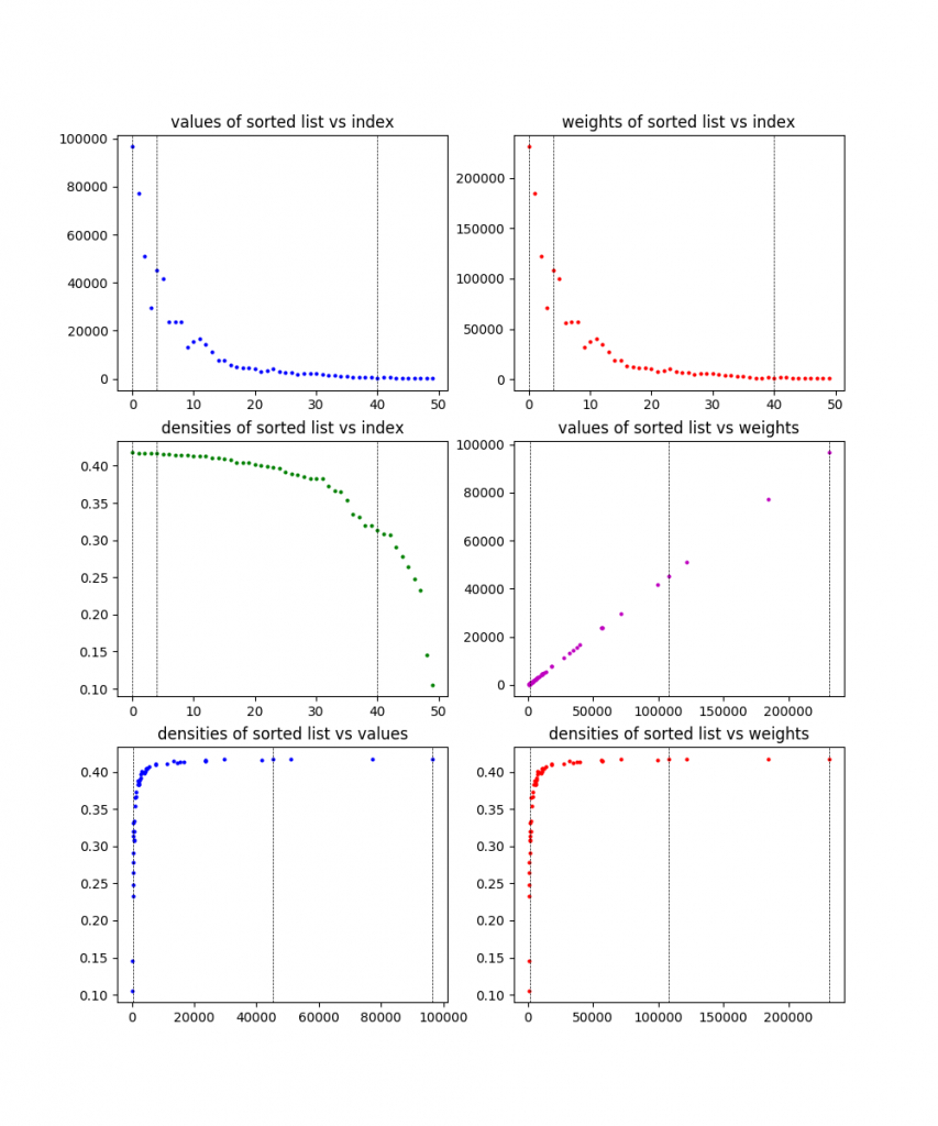
Because I like plots, I made it plot the information for each of these problems, along with the solution found (the dotted vertical lines). Here the are, in order:
30 items:

50 items:
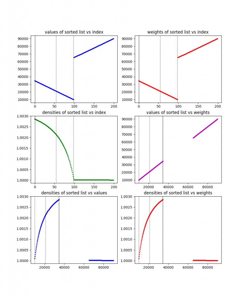
200 items:
400 items:

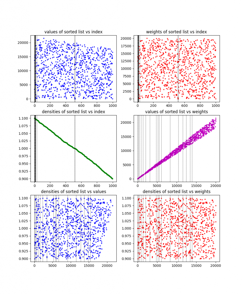
1000 items:
10000 items:
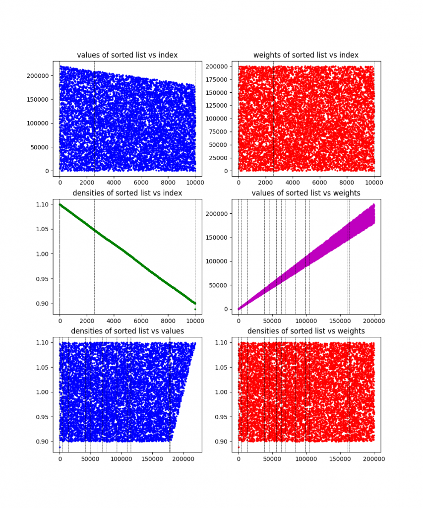
You can see from the plots that they definitely designed these problems to be wonky and have difference characteristics. To be honest, I'm still not 100% sure what the exact culprit here is that causes the 200 item problem to take so much longer than other (larger) ones. My best guess is that it has either something to do with the large gap in values (there are basically two clusters), or something about how it's clearly designed to have one of those clusters (the one that contains the solution) have decreasing density, while having the other have pretty flat density. I'm guessing whatever it is makes the linear relaxation ineffective. Maybe I'll come back to this at some point.
One other cool tweak is something my friend Max (also taking the class) came up with. Some profiling told us that the program was spending a lot of time in bestEstimate(), for the linear relaxation step. And, this makes sense: the way I'm doing it, every recursion, it has to do an O(n) operation to fill the bag (because it has to potentially go through every single item left). Instead, he did something really smart. He took the item to be considered in that recursion call, and for the linear relaxation, just filled the bag with an item of that density. Concretely, let's say there's 10 weight left in the bag and the item at hand has value 6 and weight 2. Usually you'd add that item, then go to the next, etc. Instead, you look at the density of that item (6/2 = 3), and fill the bag with that density like we did before (as if you had infinite objects at that density):
#Old version:
#linRelaxUB = valueAccum + bestEstimate(itemList[itemIndex:],roomLeft)
#New version:
linRelaxUB = valueAccum + roomLeft*itemList[itemIndex].density
The reason this works is that, remember, we're trying to bound the possible result we can get, and then if that's not as big as what we've already found a solution for, we prune. Therefore, if you overestimate the possible achievable value, the worst that happens is that you don't prune as aggressively at that point (for example, some of the time, this "extra" linear relaxed value will actually be above the best value you've found, so it won't prune it, but if you had calculated the traditional linear relax. value, that would have been below the best value and it would have pruned it). So it will still be an OS.
So, which wins out? Is not having to do that O(n) operation every recursion worth the cost of less aggressive pruning?
Hooooo yeah. Here are the times, in seconds:
Normal linear relaxation DFS: 0.012, 0.0006, 29.74, 0.279, 0.067, 6.47
And here's Max's magic DFS: 0.019, 0.0003, 16.32, 0.154, 0.042, 0.323
You can see that it outperforms it by about half for most of them, except for the 10,000 problem, where it really slams it (it also gets 60/60 of course).
One other thing that I should probably briefly mention is another tree traversal method called "Least Discrepancy Search". My friends and I still debate over one aspect of it, so what I'm going to say here should be taken with a grain of salt. LDS is similar to DFS, except the idea is that you have something called the heuristic (we'll see more of that in future posts!), which is kind of a "goal". It's in general what you want to be aiming for. So, for this problem, it seemed natural to want to always take the densest item you can. So, in LDS, you search the tree by doing a DFS, but keeping track of the number of discrepancies (not accepting an item) from the heuristic (i.e., taking every item) you've used in that search. You do this DFS search in order of increasing allowed discrepancies, starting with 0 (take every item), then 1 (take every item except for one item), etc.
The part we're debating about is what exactly counts as a discrepancy from the heuristic. For example, the way we do DFS, you do the "accept" recursion if you can (have space), and do the reject one either way. However, when doing LDS, should it count as a discrepancy if you reject the current item because you don't have space for it? It seems like you were "forced" to, so in a way it wouldn't make sense. It seems like discrepancies should be accounting for the number of choices you make that you can do but "don't make sense" according to your heuristic. That said, every tutorial I could find had the search tree organized with "accept" as the left branch and "reject" as the right, and said that the number of discrepancies is the number of right turns you take, so I implemented it that way. The results were...not impressive. It did about as good (time-wise) as plain DFS on a few problems, but much worse on others. I was kind of hoping that due to how it traverses the tree, it would at least do better on one problem (maybe that peculiar 200), but not really. It's possible I did it wrong, of course. If you know for sure, please let me know!