The breakdown of norms

Heyo again!

Today we’re gonna look at a paper called “An Inductive Bias for Distances: Neural Nets that Respect the Triangle Inequality” (2020), and go through a few parts of it I implemented.

This paper and several more recent ones attack the same problem, namely, trying to make architectures for modeling a distance metric. I’ll be using some of the more recent ones soon, and they all reference this one, so thought I’d dip my toe into this one first.

The paper could’ve been explained a little more clearly, but the idea itself is overall cool and understandable. Something I liked about it is that it has a “Factorio” feel in the sense of combining more basic elements in a clever way to get a more complex thing.

The big idea

There are some problems that can be posed in terms of finding a distance metric $d(x, y)$ between pairs of inputs $(x, y)$, and if you could find an accurate enough one, the problem would be nearly solved. The context where this comes up that I’m interested in is RL, but more on that later.

The main idea is that we’d like to make a model (and of course, it’s TYoOL 2026 so we mean a neural network (NN)) that can be trained to predict this $d(x, y)$, but ideally, also automatically enforce a few things we often expect from metrics.

You can just naively implement a “metric” by concat’ing your two inputs $(x, y)$ before shoving them into your NN model, but there’s no guarantee it’ll behave nicely in the ways we want, and in fact will provably fail some basic properties we want. Beyond that, as the paper’s title suggests, there’s also the hope that by using a type of model that is naturally good for the problem, it could speed up learning a bunch.

Definitions, basics

Some basics of metrics and norms. Skip this if you’re familiar!

A metric is a function $d(x, y): X \times X \rightarrow \mathbb R^+$ that satisfies four main properties:

• M1: non-negativity, $d(x, y) \geq 0$
• M2: definiteness, $d(x, y) = 0 \iff x = y$
• M3: triangle inequality, $d(x, z) \leq d(x, y) + d(y, z)$
• M4: symmetry: $d(x, y) = d(y, x)$

So off the bat you can kind of see why the naive NN wouldn’t work, since it probably wouldn’t obey any of these. You could get M1 for free by using a final ReLU activation, but the others seem pretty difficult to enforce with a similarly simple mod.

There are variations of this, if you drop some of those requirements. For example, if you say it doesn’t need to satisfy M2 or M4, then it’s a “quasimetric” instead of a full metric.

Also note that a metric is just defined on the ordered pair $X \times X$ for some domain $X$! It doesn’t have to be vectors, you just need to be able to assign distances to pairs of “things”.

A norm function $\Vert \cdot \Vert : X \rightarrow \mathbb R^+$ is a closely related topic: whereas a metric roughly measures a “distance between two things”, a norm is more like “a size of one thing”, and in addition, it’s only defined on vectors.

It’s also defined by a few requirements:

• N1: positive definiteness, $x \neq \pmb 0 \implies \Vert x \Vert > 0$
• N2: positive homogeneity, $\alpha \geq 0, \alpha \Vert x \Vert = \Vert \alpha x \Vert$
• N3: triangle inequality, $\Vert x + y \Vert \leq \Vert x \Vert + \Vert y \Vert$
• N4: symmetry: $\Vert x \Vert = \Vert -x \Vert$

You can probably see some parallels there, and it’s not a coincidence. You might’ve realized from the intuitive definitions I said above, wait, but can we say that the “one thing” in “size of one thing” is… the difference between two things?

And yeah, that’s exactly what a “norm induced metric” (NIM) is. If you have a norm $\Vert \cdot \Vert$ , you can create a metric from it by simply doing: $d(x, y) = \Vert x - y \Vert$. You can check that, given the fact that the norm satisfies N1-N4, the induced metric will too.

However, given that a NIM is a metric constructed in this specific way (and only defined on vectors!), it’s necessarily more restricted than a general metric. For example, it’s translation invariant: $d(x + a, y + a) = d(x, y)$, which is not necessarily true for metrics in general.

Similarly to before, relaxing some of the requirements gives you variants: if you say we don’t need N1 (i.e., you can have $\Vert x \Vert = 0$ for $x \neq \pmb 0$) then you have a “semi-norm”, and if you don’t need N4, it’s an asymmetric norm. If you induced a metric with these variants, they mostly pass on what you’d expect to the metric variants.

Finally, they use the concept of function convexity, which they call property C1. A function $f: X \rightarrow R$ is convex if for all input pairs $x, y \in X$, and scalar $\alpha \in [0, 1]$, we have $f(\alpha x + (1 - \alpha) y) \leq \alpha f(x) + (1 - \alpha) f(y)$. The usual intuition is “if you draw a line between the points $(x, f(x))$ and $(y, f(y))$, is the function $f$ always below that line in the range $[x, y]$?” Note that $x, y$ are generally vectors, but the intuition remains the same. Importantly for today, some NN activation functions like ReLU are convex.

The magic

So those are the building blocks, and now we get to the neat “Factorio” part. What they do here is build up various learnable architectures that preserve the norm/metric properties we want. They mostly focus on norms (since you can create restricted metrics from them).

Deep norms

First they show what they call “deep norms” (DN).

The first question for creating a norm is, how do you make it satisfy the triangle inequality, N3? It turns out that if a function is positive homogenous (N2) and convex (C1), then it necessarily satisfies N3!

Ok, but how do you make a NN convex? They build off of a previous paper, “Input Convex Neural Networks” (2017), which is exactly what it sounds like: NNs that are convex functions. A typical feedforward NN is a composition of functions of the input $x$. I.e., if you have activation function $\sigma(x)$ and weights layer $L_j(x) = W_j x$, the whole NN is $f(x) = \sigma(L_N( \dots \sigma(L_1(x))))$. The ICNN paper uses common rules about what types of function composition preserve convexity, to make it so the NN as a whole preserves it.

However, they need it to also be N2 and nonnegative (which the ICNN paper didn’t care about), so they modify them slightly for their needs. Let’s briefly look at the building blocks of their version.

We’ll assume our activation function $g$ is ReLU, which is convex. Therefore, given input $x$ and weights matrix $U_1$, the first layer result $h_1(x) = g(U x)$ is convex.

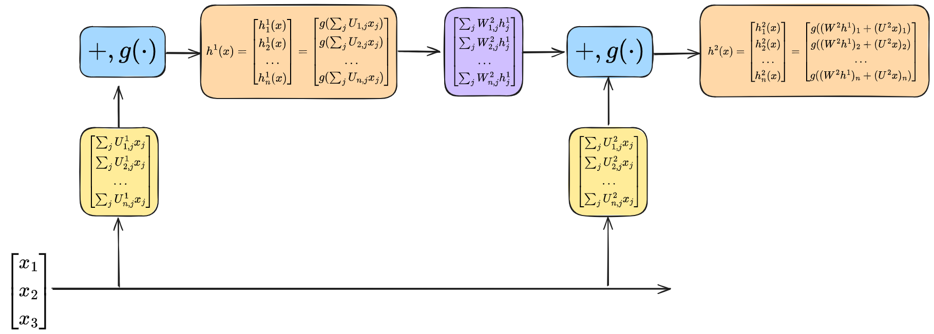
This confused me at first: $h_1(x)$ is a vector. How can a vector be convex? The key is to think of it more as a collection of functions:

\[h_1(x) = \begin{bmatrix} h^1_1(x) \\ h^2_1(x) \\ \dots \\ h^n_1(x) \\ \end{bmatrix} = \begin{bmatrix} g(\sum_j U_{1,j} x_j) \\ g(\sum_j U_{2,j} x_j) \\ \dots \\ g(\sum_j U_{n,j} x_j) \\ \end{bmatrix}\]

As long as all of the elements of these vectors remain convex (and the other properties we want), the whole thing is. Note that after this layer we also have N2 still, because $U (\alpha x) = \alpha (U x)$ and $\max(0, \alpha x) = \alpha \max (0, x)$ preserve it.

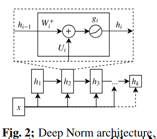
The first layer is special and simpler. The following ones use a kind of “residual” structure:

\[h_i = g(W_i^+ h_{i - 1} + U_i x)\]

I.e., $x$ is the initial input to the NN, and $h_{i-1}$ is the last layer input. Two important composition rules for convexity are being used here:

• $U_i$ is an unconstrained matrix like above, but $W_i^+$ is constrained to be elementwise nonnegative. This is because only nonnegative sums of convex functions are still convex.
• Therefore, $W_i^+ h_{i - 1} + U_i x$ is still convex in the inputs, but is $g(W_i^+ h_{i - 1} + U_i x)$? The rule here is that if you have a convex function $h(x)$, then the composition $f(x) = g(h(x))$ is only convex if $g(\cdot)$ is monotonically nondecreasing, which ReLU is.

You can see that N2 is preserved for the same reason as before – any scalar $\alpha$ passes through the affine transformations and the ReLU.

And that’s pretty much it! Then just choose the last layer, $k$, to have output size $1$, and then say $\Vert x \Vert = h_k(x)$. Since at every stage, both N2 and C1 were preserved, it’s preserved all the way to the output, and with a ReLU as the last activation function, it’s also nonnegative.

Here’s their figure showing the whole chain:

and a figure I made to help me understand the “collection of convex functions” aspect:

However, you might notice that this has given us a function that satisfies C1 and N2, and therefore N3, but not necessarily N1 or N4, so it’s therefore both a semi-norm (SN), and asymmetric, an asymmetric SN (ASN). But fear not! They have clever solutions for both of these.

First, if you have an ASN $\Vert \cdot \vert$ (note lopsided vert bars), then you can create a (symmetric) SN by doing: $\Vert x \Vert = \Vert x \vert + \Vert -x \vert$. Very clever! Any asymmetry gets canceled out by also plugging in the negative.

Second, if you have a SN $\Vert \cdot \Vert_a$, you can combine it with another full norm $\Vert \cdot \Vert_b$ (which could be just the Euclidean norm) to make it a full norm: $\lambda > 0$, $\Vert x \Vert_{a + \lambda b} = \Vert x \Vert_{a} + \lambda \Vert x \Vert_{b}$. Also clever! The problem was that we had some $\tilde x \neq \pmb 0$ such that $\Vert \tilde x \Vert = 0$. Adding, say, the Euclidean norm means that it’ll offset it with $\Vert \tilde x \Vert_2$ and it’ll no longer be zero.

There’s more they do, for example, using activation functions that “mix” the elements while still preserving stuff, but I won’t go into that today.

Wide norms

This is the second variant they do, called “wide norms” (WN). After DN, it’s a lot simpler.

The key bit is that if you already have a set of norms (including the A/SN variants), then similar to the convexity preserving ideas above, we can combine them to make new norms.

The $\max$ across the set of norms is also a norm, and any nonnegative sum is also a norm, and therefore the mean across them is a norm. They use a function called “MaxMean” which is just a weighted sum of the max… and mean. It’s also a norm, for the same reasons.

The individual norms they combine here are way simpler: for a weight matrix $W \in \mathbb R^{m \times n}$, it’s just $\Vert x \Vert_W = \Vert W x \Vert_2$, the Mahalanobis norm. So you just have a set of ${W_i}_i$, calculate the Mahalanobis norm, and then calculate the maxmean across them:

\[\Vert x \Vert = \text{maxmean}_i \big( \Vert W_i x\Vert_2 \big)\]

That’s it!

You can see that by default, it’s symmetric (since the negative of an input cancels with itself), and whether it’s a proper norm or a SN depends on $W$ – if it has a nullspace, then it necessarily has $x \neq \pmb 0$ that map to zero and it’s a SN. You can get this if it’s square and singular, or just shorter than it is wide. They similarly use a couple tricks to make them able to support asymmetry.

Neural metrics

Neural metrics are their last architecture. They’re a modification you can put on top of either wide or deep norms to make them more expressive than NIM can be on their own. However, I won’t do them today. Let’s see some experiments!

Experiments, results

They do a few different experiments, but today I’m just gonna show the first set of them that I reproduced.

This is from section 2.5, “modeling norms in 2D”. The idea here is what it sounds like: we’ll create a few artificial norms in 2D space, and then see if these special models can learn those norms, and how they do compared to simpler ones.

To create the norms, they use the fact that there’s a one-to-one equivalence between any (bounded, open) convex set in $\mathbb R^n$ and some (possibly asymmetric norm). This is an unnecessarily fancy way of saying: since a norm tells us the size of a given vector in $\mathbb R^n$, then if we draw a (convex) shape around the origin, we can say that the points on its perimeter are where that norm is equal to one, and now we’ve defined a norm!

To make them, they do a little procedure where you sample some means and variances for Gaussian clusters, and then sample some points from those clusters. Then you take the convex hull of all those sampled points, and that’s your norm:

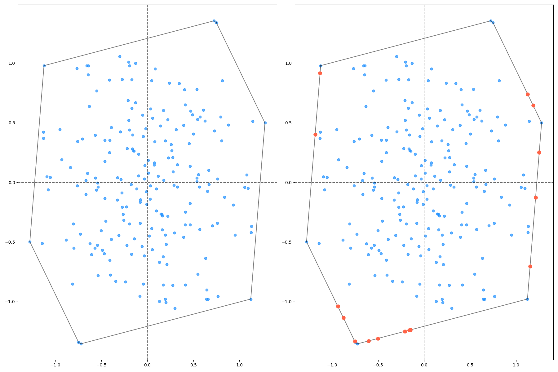
These will be asymmetric by default, but we can then also make symmetric versions from them.

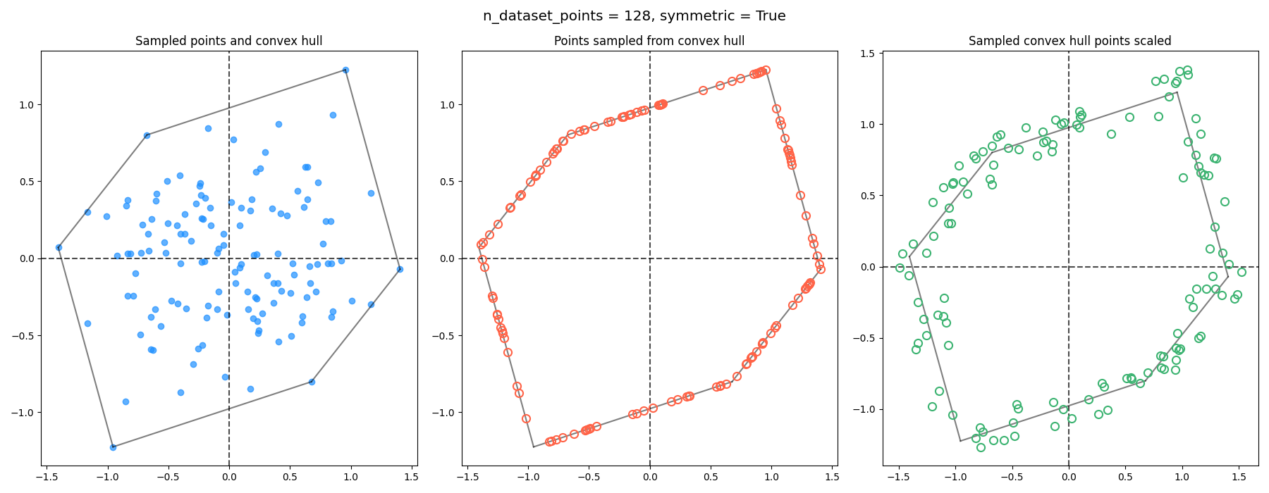
This is how the norm is formed, but what’s the actual training data? For this, they sample some $500$ points around the convex hull perimeter (in red below). Remember that under the norm we want to learn, these have magnitude one, which will be the true norm label. Then, from these, they sample either $k = 16$ or $k = 128$ points, which will form the training data. For each of these train data points, they scale it by a number in $[0.85, 1.15]$ (giving the green points in the figures below), which will then be the true norm label for these points.

The original $500$ points will the test dataset that they’ll use for early stopping. So it’d look like so:

Symmetric example:

Asymmetric example:

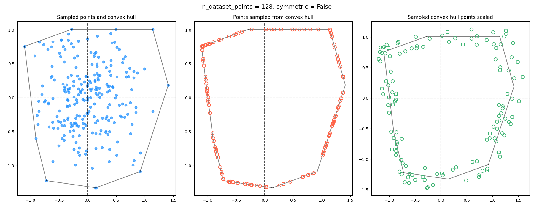
There are a few funky things about this dataset setup. Most notably, the training datasets are tiny! I don’t think I’ve ever used a training dataset of size $16$ before this. Further, the train/test sizes are totally reversed: usually you hear of something like an 70/30 train/test split, but this is either 128/500 or 16/500. Lastly, we usually split the train/test from the same dataset, but this is specifically done with them being different. What gives?

I think the point of all this is that they want to highlight how their models extrapolate and generalize in a way that other models don’t. By using really small training sets, the inductive bias of these models will prevent it from doing anything too crazy when extrapolating, while an unconstrained model can just go bonkers.

Anyway, onto the results. They show results for four norms: square norm (i.e., $L_\infty$) diamond norm (i.e., $L_1$), and an example of one symmetric and one asymmetric norm. For each, they train with dataset sizes of $k = {16, 128}$. For each of those, they show results for {Mahalnobis norm, Deep Norm, Wide Norm, Unconstrained MLP}.

Here are my results for $k = 16$:

In the left plot you can see the target norm and the $k$ points that form the train dataset. In the other columns you can see the predictions from each of the different models. On each, the contours of the true norms are shown at values of ${0.5, 1.0, 1.5}$ in different colors. The contours at those same norm values that are predicted by the model are shown in black and labeled with the contour value (i.e., the contour labeled $1.5$ are the points that the model predicts have a norm of $1.5$). Obviously, we’d like the black contours to be on top of the colored ones. Lastly, the background color shows the predicted norm values at all points (which you can read from the shared legend).

Alright, so what are the high level takeaways from these results?

• The Mahalanobis norms are… doing the best they can, but they’re fundamentally limited to a shape that just doesn’t match most of them (it’s not too bad for the random symmetric norm though!)
• Overall, it seems like my Deep Norms are doing the best at a glance
• The MLP doesn’t actually do too bad in terms of its $1.0$ contours matching the true ones, but you can see that it does quite badly for the other contours. More on that below.

Same results, but $k = 128$:

Big takeaways:

• Mahalanobis is about the same, since it was already about as good as it can get with $k = 16$
• DeepNorm is now nearly perfect
• The WideNorm ones still aren’t great for the random generated norms
• The MLP is nearly perfect at all contours for all norms (more on this later)

What’s goin on with them numbers? Discussion

A little bit of the bad extrapolation?

If we look at the $k = 16$ results for the symmetric and asymmetric norms:

This is the best “here’s what we wanted to see!!” figure I think we’re gonna see today. All the models were trained only on points around the $1.0$ contour. As I mentioned above, the MLP isn’t doing too bad for the $1.0$ contour, but it isn’t great with the others, which is the type of behavior folk-ML-wisdom says we should generally expect with NN’s when they extrapolate.

In contrast, you can see that the paper’s norm models scale perfectly to inputs of other magnitudes (as they must, by design).

…but the MLP is actually not that bad?

Despite those examples above, the MLP is actually not that bad, even for the $k=16$ results. And for the $k = 128$ results, it’s doing downright amazing!

It’s basically exactly on par with DeepNorm.

So… what’s going on? If we look at their corresponding figures:

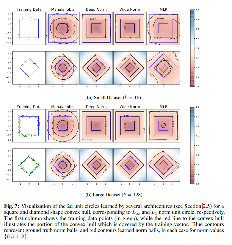
and

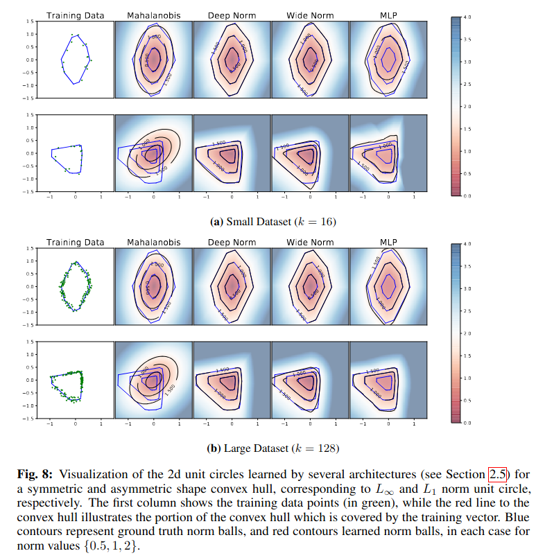
Their MLP examples are really bad for the square and diamond norms, even for $k=128$!

This is… a little suspicious. When I try to implement something, if my results for the paper’s method aren’t as good as the paper reports, it’s very likely I messed up something, or they left out a crucial implementation detail (very common unfortunately…). Not ideal, but understandable. However, when I get way better results for the very simple baseline method they’re comparing to, it kind of looks like they’re sandbagging.

My wide norms suck?

My wide norms obviously aren’t good compared to theirs. I suspect I may have implemented something slightly wrong. They’re clearly not completely broken, since they can learn the square and diamond norms very well, and learn the other ones reasonably. But they’re pretty wonky and don’t look nearly as nice as theirs.

There are a lot of implementation details that I didn’t talk about, that they mention in the text but are pretty vague about in terms of what they actually used. So I wouldn’t be surprised if I either messed something up, or there’s some little thing they didn’t say. Maybe I’ll look into this more another time.

Their losses are really really small?

They show the test dataset MSE loss (at a few different target norm values) across the results, like this:

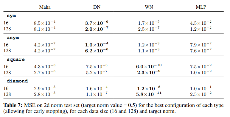
I made the same results for mine:

Target Norm $1.0$:

\[\begin{array}{lrrrrr} \text{} & \text{Mahal.} & \text{DN} & \text{WN (Asym)} & \text{WN (Sym)} & \text{MLP} \\ \hline \pmb{\text{Square}} & & & & & \\ \text{16} & 1 \times 10^{-2} & \mathbf{1 \times 10^{-4}} & 2 \times 10^{-3} & 7 \times 10^{-4} & 9 \times 10^{-4} \\ \text{128} & 1 \times 10^{-2} & \mathbf{3 \times 10^{-6}} & 8 \times 10^{-4} & 3 \times 10^{-5} & 4 \times 10^{-5} \\ \hline \pmb{\text{Diamond}} & & & & & \\ \text{16} & 1 \times 10^{-2} & 3 \times 10^{-4} & \mathbf{4 \times 10^{-6}} & 3 \times 10^{-3} & 1 \times 10^{-3} \\ \text{128} & 1 \times 10^{-2} & 6 \times 10^{-6} & \mathbf{1 \times 10^{-6}} & 5 \times 10^{-5} & 2 \times 10^{-5} \\ \hline \pmb{\text{Sym}} & & & & & \\ \text{16} & 3 \times 10^{-3} & 5 \times 10^{-4} & 4 \times 10^{-3} & \mathbf{5 \times 10^{-4}} & 1 \times 10^{-3} \\ \text{128} & 3 \times 10^{-3} & \mathbf{7 \times 10^{-6}} & 2 \times 10^{-3} & 7 \times 10^{-5} & 1 \times 10^{-5} \\ \hline \pmb{\text{Asym}} & & & & & \\ \text{16} & 2 \times 10^{-2} & 9 \times 10^{-4} & 4 \times 10^{-3} & 2 \times 10^{-2} & \mathbf{6 \times 10^{-4}} \\ \text{128} & 2 \times 10^{-2} & 1 \times 10^{-4} & 3 \times 10^{-3} & 2 \times 10^{-2} & \mathbf{1 \times 10^{-5}} \\ \hline \end{array}\]

Target norm $0.5$:

\[\begin{array}{lrrrrr} \text{} & \text{Mahal.} & \text{DN} & \text{WN (Asym)} & \text{WN (Sym)} & \text{MLP} \\ \hline \pmb{\text{Square}} & & & & & \\ \text{16} & 3 \times 10^{-3} & \mathbf{4 \times 10^{-5}} & 5 \times 10^{-4} & 2 \times 10^{-4} & 5 \times 10^{-3} \\ \text{128} & 3 \times 10^{-3} & \mathbf{7 \times 10^{-7}} & 2 \times 10^{-4} & 8 \times 10^{-6} & 2 \times 10^{-4} \\ \hline \pmb{\text{Diamond}} & & & & & \\ \text{16} & 3 \times 10^{-3} & 8 \times 10^{-5} & \mathbf{1 \times 10^{-6}} & 7 \times 10^{-4} & 2 \times 10^{-2} \\ \text{128} & 3 \times 10^{-3} & 2 \times 10^{-6} & \mathbf{3 \times 10^{-7}} & 1 \times 10^{-5} & 2 \times 10^{-4} \\ \hline \pmb{\text{Sym}} & & & & & \\ \text{16} & 7 \times 10^{-4} & 1 \times 10^{-4} & 1 \times 10^{-3} & \mathbf{1 \times 10^{-4}} & 3 \times 10^{-2} \\ \text{128} & 7 \times 10^{-4} & \mathbf{2 \times 10^{-6}} & 5 \times 10^{-4} & 2 \times 10^{-5} & 8 \times 10^{-5} \\ \hline \pmb{\text{Asym}} & & & & & \\ \text{16} & 6 \times 10^{-3} & \mathbf{2 \times 10^{-4}} & 9 \times 10^{-4} & 5 \times 10^{-3} & 2 \times 10^{-2} \\ \text{128} & 6 \times 10^{-3} & \mathbf{4 \times 10^{-5}} & 7 \times 10^{-4} & 5 \times 10^{-3} & 9 \times 10^{-5} \\ \hline \end{array}\]

Target norm $1.5$:

\[\begin{array}{lrrrrr} \text{} & \text{Mahal.} & \text{DN} & \text{WN (Asym)} & \text{WN (Sym)} & \text{MLP} \\ \hline \pmb{\text{Square}} & & & & & \\ \text{16} & 3 \times 10^{-2} & \mathbf{3 \times 10^{-4}} & 5 \times 10^{-3} & 2 \times 10^{-3} & 5 \times 10^{-3} \\ \text{128} & 3 \times 10^{-2} & \mathbf{6 \times 10^{-6}} & 2 \times 10^{-3} & 7 \times 10^{-5} & 3 \times 10^{-4} \\ \hline \pmb{\text{Diamond}} & & & & & \\ \text{16} & 3 \times 10^{-2} & 7 \times 10^{-4} & \mathbf{1 \times 10^{-5}} & 6 \times 10^{-3} & 2 \times 10^{-2} \\ \text{128} & 3 \times 10^{-2} & 1 \times 10^{-5} & \mathbf{3 \times 10^{-6}} & 1 \times 10^{-4} & 8 \times 10^{-5} \\ \hline \pmb{\text{Sym}} & & & & & \\ \text{16} & 7 \times 10^{-3} & 1 \times 10^{-3} & 9 \times 10^{-3} & \mathbf{1 \times 10^{-3}} & 3 \times 10^{-2} \\ \text{128} & 6 \times 10^{-3} & \mathbf{2 \times 10^{-5}} & 4 \times 10^{-3} & 1 \times 10^{-4} & 7 \times 10^{-5} \\ \hline \pmb{\text{Asym}} & & & & & \\ \text{16} & 5 \times 10^{-2} & \mathbf{2 \times 10^{-3}} & 8 \times 10^{-3} & 5 \times 10^{-2} & 2 \times 10^{-2} \\ \text{128} & 5 \times 10^{-2} & 3 \times 10^{-4} & 6 \times 10^{-3} & 5 \times 10^{-2} & \mathbf{3 \times 10^{-4}} \\ \hline \end{array}\]

I know my results aren’t as good as theirs, but… their MSE values are really small. Like, if you look at my results for $k = 128$ with the diamond norm, they look about as good as I can see by eye and the table above says they only get down to a MSE of $\approx 10^{-6}$. They’re hitting numbers in the range $10^{-8} - 10^{-11}$. It makes me wonder if they’re doing something different.

Pretty sloppy in a lot of places

You might’ve seen in the figure captions above that they said:

[!NOTE] Fig. 7: Visualization of the 2d unit circles learned by several architectures (see Section 2.5) for a square and diamond shape convex hull, corresponding to L∞ and L1 norm unit circle, respectively. The first column shows the training data points (in green), while the red line to the convex hull illustrates the portion of the convex hull which is covered by the training vector. Blue contours represent ground truth norm balls, and red contours learned norm balls, in each case for norm values {0.5, 1, 2}.

My emphasis. They say they do norm values including $2$ there, but the figures themselves and other text says $1.5$. Okay, not a huge deal, but messy. Similarly, what “red line” ? I don’t see any red line in the figure.

There are a bunch more things like this. I think it’s a bit analogous to “code smell”, but for research writing. It doesn’t change any results itself, but what are the chances they were only sloppy here in the places you can see, and only making aesthetic mistakes?

For example: as a spoiler, in a future post I’ll be going over this paper (“IQE”). It’s on the same topic so they compare to this post’s paper. I didn’t mention it above, but in the DeepNorm section they mention using a type of activation that’s specifically not elementwise, in that it can “mix” inputs. They call it “MaxReLU” and for each pair of inputs $(x, y)$, it does:

\[\text{maxrelu}(x, y) = [\max(x, y), \alpha \cdot \text{relu}(x) + \beta \cdot \text{relu}(y)], \ \ \alpha, \beta \geq 0\]

Notice anything wrong? I didn’t! But in the IQE paper they point out that while MaxReLU is indeed C1 and N2, it can actually be negative, due to the $\max$, and the final output needs to be nonnegative (as all norms must be).

Again, this doesn’t seem like it was a problem for either them or me (I actually used regular ReLU here, as IQE suggested doing for a fix), and we’d probably expect it to try to learn to make those outputs positive anyway. But it’s a little worrying, still.

Adieu

Anyway, enough complaining. The paper is still overall very cool, and I learned a lot in going through it and implementing some of it.

I may come back to it another time and implement the remaining part (Neural Metrics) and other experiments, but for now, there are other ones I want to move onto.