[latexpage]
A while ago, I did a post on beating OpenAI games using neuroevolution (NE). Go read that if you're interested, but here's the gist: a typical strategy for training an agent to beat those games is to have a neural network (NN) play the games a bunch, and then improve the weights of the NN using a reinforcement learning algorithm that uses gradient descent (GD), and it of course works pretty well.
However, an alternative to those methods is to use a gradient free method (which I'll call "GD-free"), like I did in that post: you try a bunch of random changes to the NN's weights, and only keep the resulting NNs that play the game well. That's the "evolutionary" aspect of it, and using methods like that to create NNs is often called "neuroevolution" (NE).
That's one difference from a typical GD method. Another is that I didn't just have it change the weights, I also gave it the ability to add nodes, add weights, or remove weights. So it starts from scratch (just input and output nodes, and a bias node), and builds successful NN's from scratch (a pretty common strategy in NE).
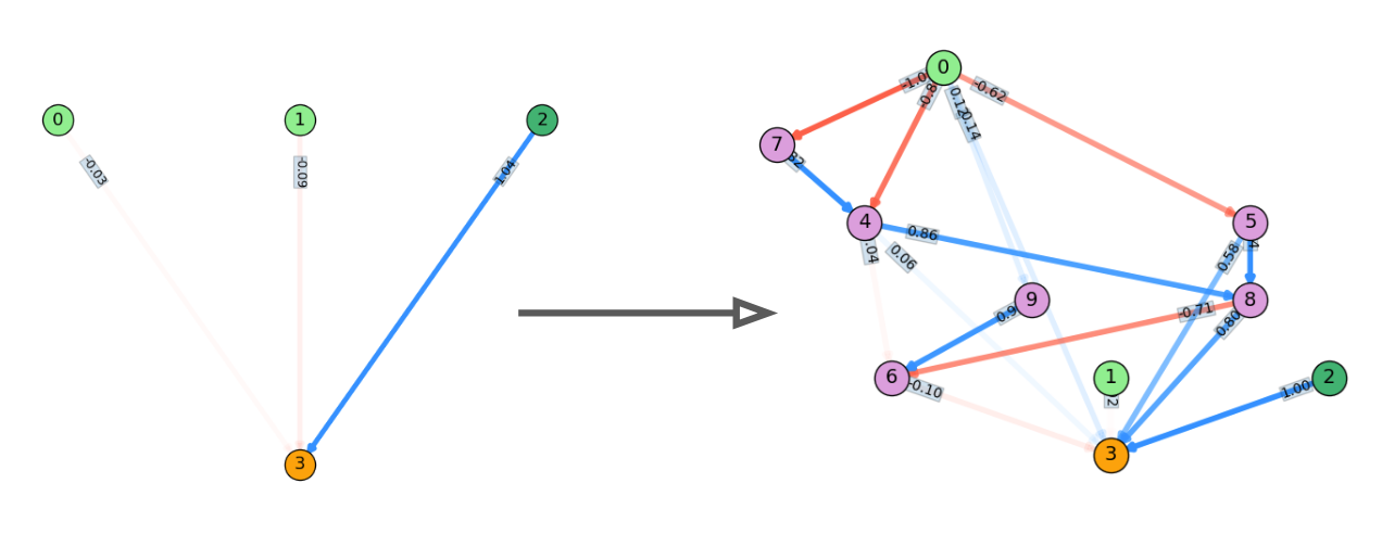
So, those worked for those simple games, but the larger reason I'm interested in NE is because I think it potentially offers an exciting path forward to more interesting AI. The way we do typical deep learning is to take a massive NN, and then improve it using GD for the task at hand. It obviously works really well, but I worry that it's not really scalable to general problems; even AlphaZero can be trained to learn varying and incredibly complex games, but it doesn't really learn any general concepts and doesn't reuse similar stuff it learns in one environment in another environment.
(Addressing this problem is a huge research area, so this isn't some really insightful revelation I'm making here :P)
In contrast, lots of impressive structures you see in the world are modular and hierarchical, which naturally lends itself to reuse and generality. For example: with complex electronics and computers, you start with a handful of very simple components, and combine them in clever ways to make "meta components", or "modules", that you can treat like a black box that does a specific task. You figure out how to wire together a couple transistors and a few resistors, and now you've got a NAND gate. You wire some of those together to make an AND or OR gate, then wire those together to make a single bit half adder, etc., and you eventually get a computer (more on this below).
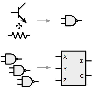
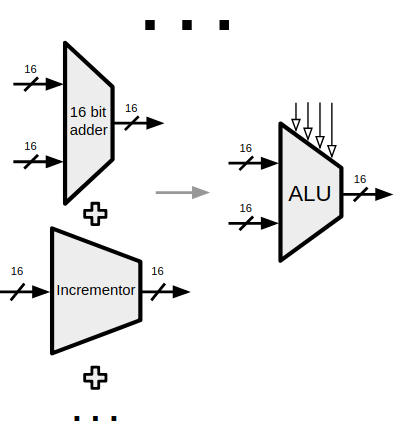
 My point is that it seems like you eventually need some concept of modularity to do the really cool stuff. And of course, here again, there's a tonnnn of research being done on this topic, which I'm really interested in. So here's an extension of what I did last time!
There are two main additions here. The first is that here, I use both the evolutionary strategy and GD. Last time, the only way to change the weights was for them to randomly mutate. It...worked, but really slowly: finding an acceptable set of even just 12 weights is still a large parameter space to search randomly. So, in this article, I'm still letting it mutate the NN to add/remove nodes/weights, but I'm letting it find the best weights it can for its current architecture by training it with GD. This turns out to be much faster, as you'll see.
The other addition is an attempt at modularity. Last time, I was just adding typical NN nodes that sum their inputs and then apply a nonlinear function to that sum. Here, to make it modular, I made it so it can save a successful NN as a discrete module, and then later, instead of adding a regular NN node, it can add the whole module!
First, let's see how much GD improves the speed. In anticipation of the modular aspect, the task I made the agents do was to design classic logic circuits. This was certainly inspired by the fact that my friends and I were taking the famous nand2tetris course. In it, you start with just a NAND logic gates, and combine them to make other basic gates. Then you combine those to make bit adders, then byte adders, then an ALU, and eventually a CPU (the course was amazing, well explained, and I highly recommend it).
However, it's also a great environment to try and experiment with modularity!
So those are the "agents" I'm trying to build for this post. In contrast to last time, where they were intended for RL problems and therefore just returned rewards from playing, here there are correct answers, so it's basically a supervised learning problem. Here's an overview of what happens:
- The initial population are all blank NNs, with just input, output, and a bias atom (which always has a value of 1.0):
- Evolution starts: every generation, each individual NN is trained on the problem at hand for $N_{train}$ iterations to improve their weights. Then, the trained NN is tested on a smaller $N_{eval}$ number of iterations, which is used to get its fitness function (FF).
- Then, the population is sorted by FF, and the top N of them are kept and the rest thrown away. These top N are cloned to make a full sized population again.
- Next, every individual of this new population mutates (add a node, add a weight between two nodes, remove a weight) with some probability, and the steps 2-4 are repeated until the top FF is above some threshold considered solved.
How does it work?
Not bad! Here's the progression of a NAND gate getting constructed:
an OR gate:
an AND gate:
There are a few things you might notice. One is that the NN's are wayyy more complicated than they theoretically need to be. This has to do with the hyperparameters used to construct them; in general, you can make it proceed more slowly, and it will end up with simpler NN's (more on this below). Another thing is that some of them look a little unbelievable. For example, an OR gate is symmetrical with respect to its two inputs x and y, but the final NN above is distinctly asymmetric. When I first saw it, I thought, hey, that can't be right. But do the math out (using tanh at the outputs of the purple nodes), and you'll see that it does!
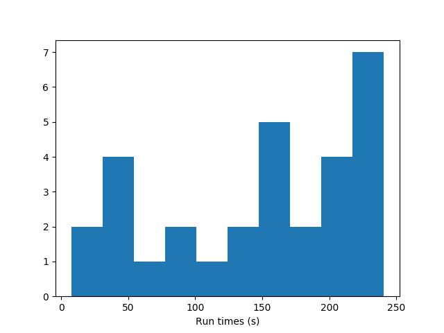
Let's also compare this to the previous method (GD-free), doing the same task of building a NAND gate. Here, I'm comparing the FF of each with respect to the total wall time because the methods require very different hyperparameters and it would be meaningless to compare the FF vs generations. Further, because there's a decent amount of variance in how long a full evolution takes (for both methods), I run them each for 30 full evolutions and plot a histogram of their run times.
GD-free:
GD:

It's lots faster, because it doesn't have to figure out the weights randomly. GD can't deal as well with discrete choices (like adding nodes/weights), but it really slams it when there's a simple solution where the weights just have to be tuned correctly. Note that for both of these, I set a limit on the runtime of each evolution of 4 minutes, so for the GD-free one, a bunch of them don't even finish in that time.
Okay, so that's that part. The modular part is a bit more complex.
I wanted the algorithm to solve a simple problem like the NAND gate, but then be able to package it into a discrete module that could be inserted into another NN as a mutation, in addition to regular nodes. To differentiate them from regular NN nodes, but also emphasize the discreteness of these constructed modules, I wanted a different name than "node", so I call one of these modules an "atom". I want to emphasize that although they're originally built from regular nodes, an atom is just meant to act as an input/output function once it's inserted into another NN. More on that below.
To be able to "package" the atom, the atom is stored as a json file. The simplest, starting one, the original NN node, is just:
{
    "Name": "Node",
    "N_nodes": 1,
    "N_inputs": 1,
    "N_outputs": 1,
    "atom_function_vec": [
        "tanh(a_0)"
    ]
}
The really important part is the bottom, where it shows the function of the atom. The program knows to look for a single input, which it will call a_0, and then apply tanh() to it. The summing you typically expect for a node is expected to be handled external to the node/module.
This functional form lets me do two cool things!
First, it lets me compose a bunch of atoms via their functions. When the NN is created, the program starts at the graph input/bias nodes, and uses sympy to plug in the placeholder symbols $i_0, i_1, i_2, ... $ to the input nodes' atom functions. The outputs of these input nodes are then propagated to the atoms that they output to, where each atom is collecting a vector of inputs (which are all in terms of the original input $i_n$ symbols now). When it's one of those atoms' turns to propagate, it sums its input vector, and plugs it into its' atom function, and the process is repeated until the final output nodes of the NN have their values.
This is a bit tricky, so here's a practical example. I'll build a simple NN for a NAND gate and show it and its corresponding total function (i.e., what the output node outputs as a function of the input to each input node, $i$) as it gets added to!
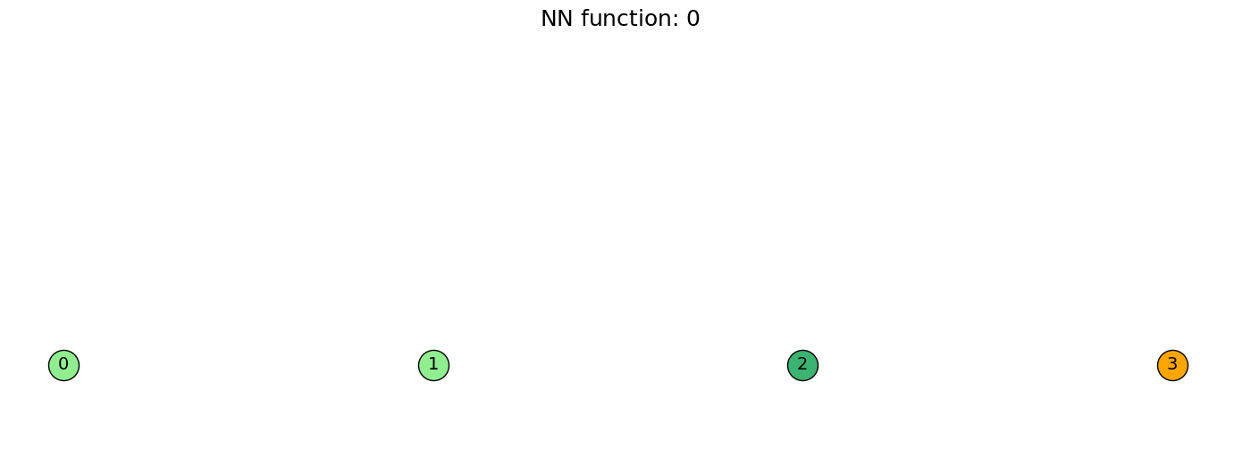
Starting with the blank NN, we have the two input nodes (light green), the bias node (dark green, value always 1.0), and the output node (orange). The default output (with no inputs) of every (non-bias) node is 0, so the value of the orange output node is 0 no matter what inputs you give the NN.
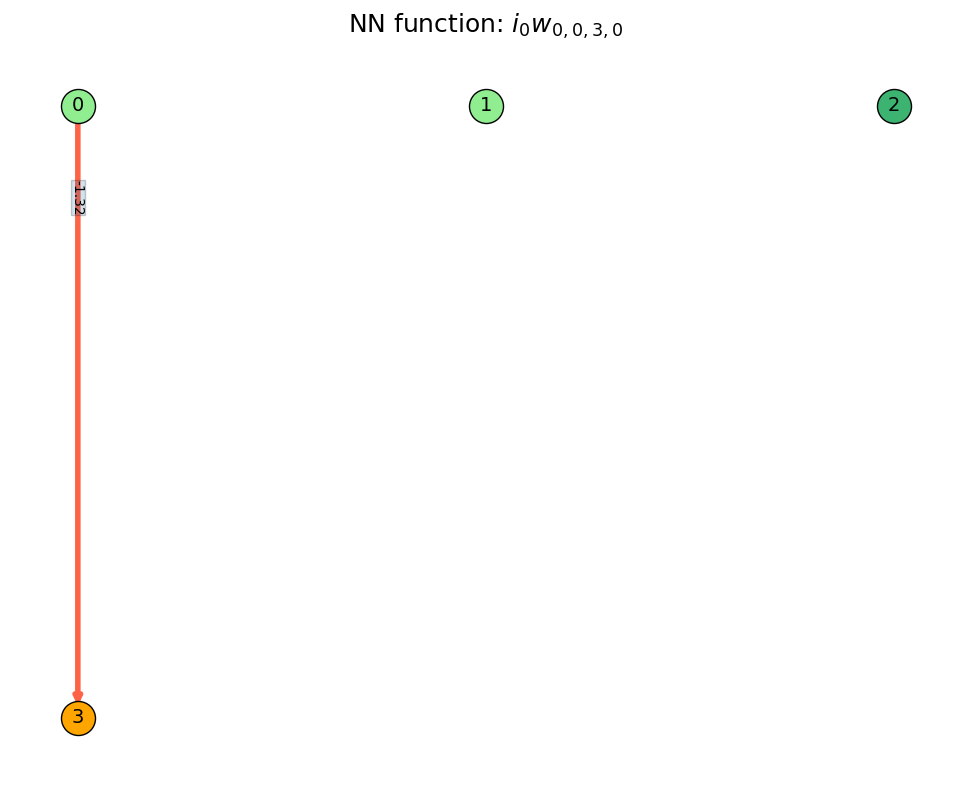
A weight is added from 0 to 3. $i_0$ represents the input to node 0, and weight $w_{0,0,3,0}$ is the weight from node 0 to 3 (ignore the other 0's for now, we'll get to that later). Note that it's still linear at this point, because neither input or output nodes apply a nonlinearity to their summed inputs.
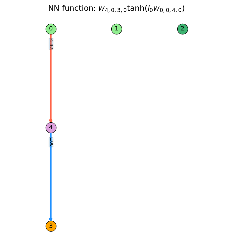
Next, a regular node (atom) is added in between nodes 0 and 3. It does apply tanh() to its summed inputs, but it's still only getting input from node 0.
A weight is added from node 1 to 4, so it now gets inputs $i_0$ and $i_1$, with their corresponding weights.
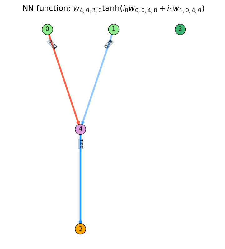
Lastly, the bias node is added. Note that in the function, its value is 1.0, because it doesn't take inputs, it just acts as a constant.
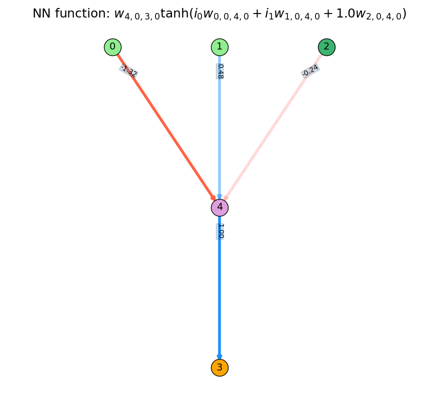
The specific values of the weights are untrained, but this has the form of a simple NAND gate.
So that's one part. While this may seem trivial, now we can save it as its own discrete atom in a json file:
{
    "Name": "Atom_NAND",
    "N_inputs": 2,
    "N_outputs": 1,
    "atom_function_vec": [
        "1.0*tanh(-1.32449531555176*a_0 + 0.480630934238434*a_1 - 0.237370386719704)"
    ]
}
Now let's say we have a problem where we need to (for some reason), connect 10 pairs of NAND inputs (so, 20 inputs) to 10 corresponding outputs. Doing this by just adding simple atoms and using GD as above would be a pretty hard problem. With our saved NAND atom though, here's a solution:

There are of course a whole new set of problems that come along with this, but I'll mention them later.
The other cool feature of this modular method is that it easily lets you still tune the weights of the network that aren't in atoms. For example, with the NAND gate I constructed and saved above, if you trained it to have good weights before saving it, you'd probably never want those weights to change once you inserted it into another NN; you'd want the NAND atom to act as nothing but a set input/output function, while you'd want to tune the weights around it.
To illustrate this, let's insert the NAND atom from above, and look at the resulting NN output function:

Note that, because it was inserted as an atom here, although it internally has weights, they're represented as their numerical values, whereas the weights outside the atom are still variables. This means that when I run gradient descent, it only affects the weights outside atoms! You could certainly accomplish this by instead carefully masking the weights and choosing only the non-atom ones to be updated, but this works really nicely.
So, how well does it actually work? Well... let's just say that this part was less of a success. However, it was really a first stab at it, so there are lots of things to try. What I tried doing was the following. The mutation that adds an atom can now add either a simple node, or a "complex atom", meaning one that has been saved previously (in a directory that it looks in), with some probability, $p_{complex atom add}$.
The perfect example to try it on is a MUX gate, which basically has two main inputs, and also a third input that determines which of the two main inputs to use as the output. It's perfect for this because it can be constructed entirely out of NAND gates:
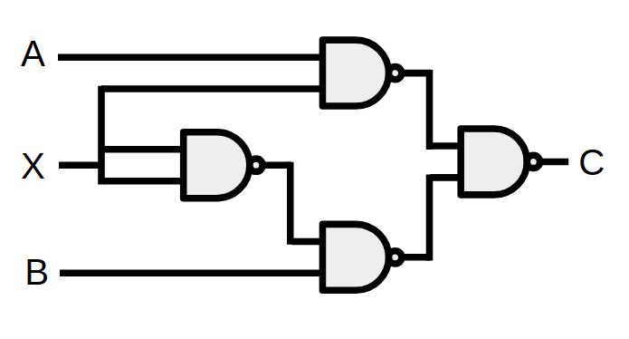
So if you crank up this $p_{complex atom add}$, it will insert them...
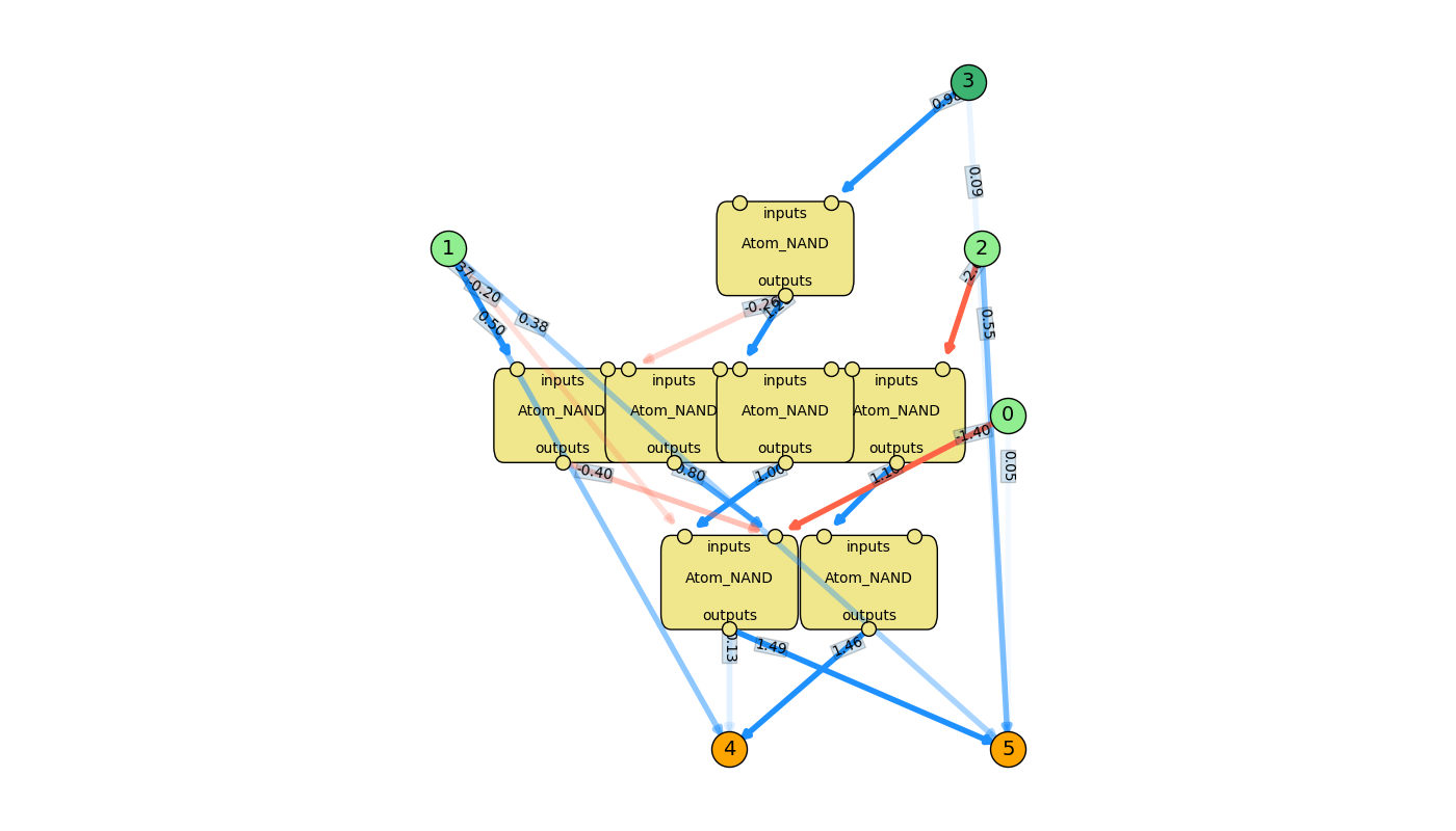
...but not really effectively, and it makes a horrible franken-network. The FF never gets really good, despite what hyperparameters I use. In fact, the problem is still simple enough that if I just have it build it without these NAND atoms, it still gets it:
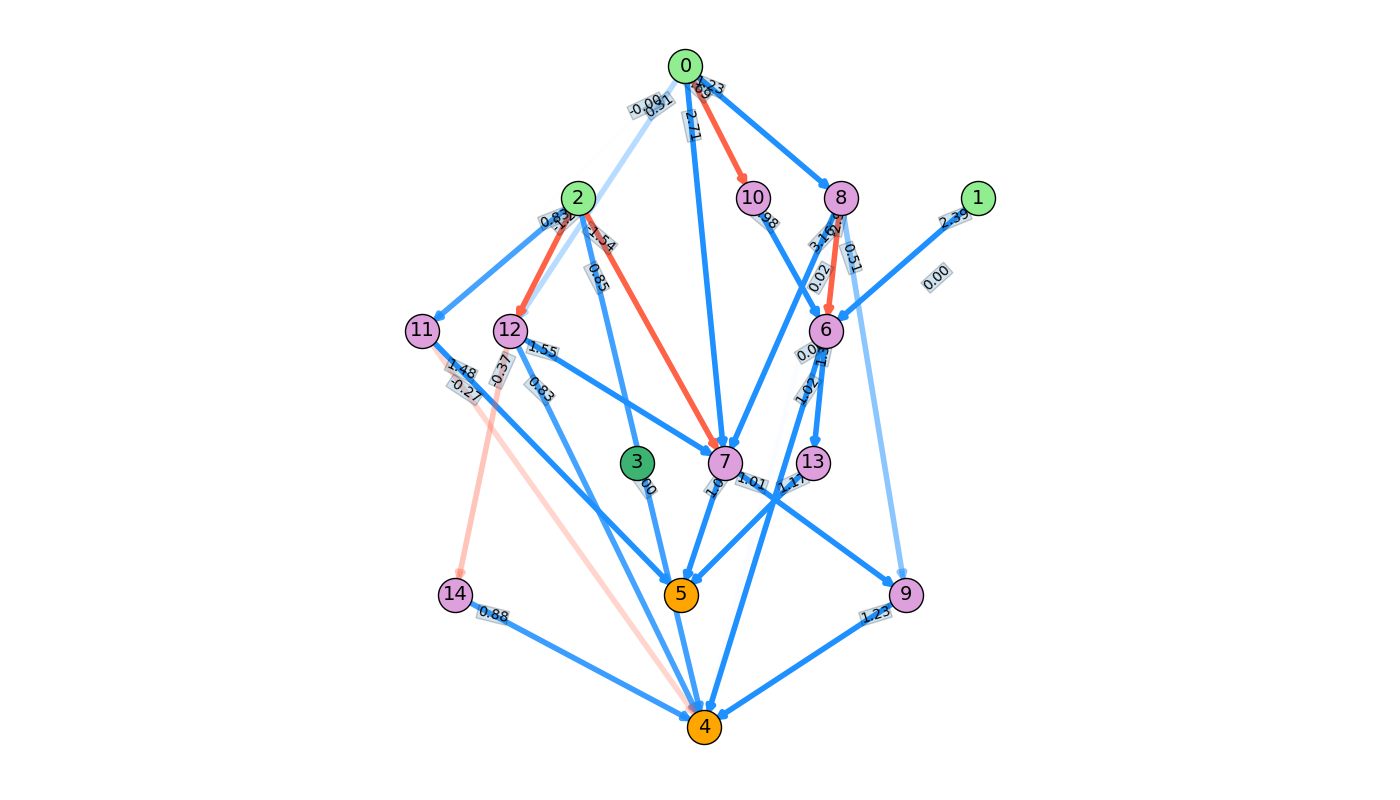
I think there are two main barriers to getting this working. The first is that, even if you have the perfect atom for a given task (like, let's say you have a single bit XOR gate, and you want to make a 16 bit XOR), it's still not trivial to actually hook them all up! The program has to insert that many XOR atoms, and then for each one, hook up two input nodes to the atom's inputs, and the atom's output to the output node of the NN.
The other problem is part of a larger mystery to me. I was kind of naively hoping that, like in our nand2tetris course, if I had it produce and save the NAND, OR, AND, XOR gates, I could them stick them in that directory and have it start making the next stage of more complicated ones (adders, incrementors, etc) out of those basic ones, by giving it all the options and waiting long enough. Of course, if the simpler one above (where it had a single option) didn't work, this one really didn't work. It turns out that when it has all these options, it becomes really unlikely that it's going to choose the correct subset of them and wire them up correctly.
The reason it's part of a larger mystery to me is that another very successful and relatively modular system is our gene expression/RNA transcription. We have these relatively discrete parts (genes, codons, proteins) that combine in just the right ways to create crazy higher order things, but I don't know (probably cause I don't know enough developmental bio!) how evolution managed to create a system that chooses the right combination of things, when there's such a huge number of combinations.
Well, that's all for now. I have some other ideas to improve these parts, which I'm sure I'll write about soon. Below are some details, so check those out if you want to see the nitty gritty. Thanks for reading!
Details:
Here are some interesting details I've left for the bottom, because talk about learning rates and hyperparameters is a lot less exciting that flashy gifs! Read on if you're interested.
Looking forward, and literature
This has, of course, been tried before in various formulations! I'm not going to pretend to be original when I'm not. Modularity is a big, promising field, so there are lots of attempts at answering questions like "How do you get modularity to arise effectively and automatically?" and "Is modularity (in our brains, for example) a side effect of other things, or a necessary component for that structure?" For example, there's good evidence that local connectivity arises out optimal wiring of neurons in the brain. There's also evidence that modularity lends to better selection fitness in changing environments.
Some papers I've read regarding that stuff:
Global optimization of cerebral cortex layout
Principles of modularity, regularity, and hierarchy for scalable systems
Wiring optimization can relate neuronal structure and function
The evolutionary origins of modularity
It seems like most attempts at doing the type of stuff I did fall into a couple camps. A very common one you see these days are treating whole layers of a NN as the "modules", and then adding them. This actually makes several of the problems I encountered considerably easier; if you assume each layer is fully connected to the next one, you don't have to deal with the "I have the right components, but how do I make sure they're fully connected?" problem. Additionally, it's just a much simpler formulation: each layer has a type, and a couple other hyperparameters (like the stride/# filters/etc for CNN's, a classic use case). In these, it's very common to do the paradigm I used here of 1) Build network 2) train/test 3) select somehow 4) repeat.
In that vein:
Large-Scale Evolution of Image Classifiers
Neural Architecture Search with Reinforcement Learning (very cool, I'll be talking about this one in the future!)
Designing Neural Network Architectures using Reinforcement Learning (very similar, also very cool)
Another tact is explicitly making sub-modules, and then having another "controller" (or other lingo) NN decide when to use them. They've used these in things like first person shooter games, where they'll have a "shoot" module, a "explore" module, etc. It's cool, and probably actually has good practical performance, but I don't like how it just kind of needs to be human assigned on a different level.
Comparing the GD method to GD-free method
It's a bit difficult to compare them. First, it seems like the GD and GD-free methods have very different optimal hyperparameters, but the process is both lengthy and so stochastic that it's hard to find them. Additionally, because the runtime varies a lot, it's only meaningful to run the same evolution repeatedly to form a distribution of the runtimes, and then look at their mean. And, if a typical run takes an average of ~2 min, and I want a distribution of 30, we're looking at an hour to test one set of hyperparameters (I tried some Bayesian Optimization, but it was just too noisy to pick up anything with the number of runs I was doing).
Second, the GD method needs a bunch of training/test samples (I typically used 300/30). On the other hand, the GD-free method doesn't need to train at all, it just needs to evaluate how good the network is. So for the evaluation step (for both methods), I could do a "deterministic" way where instead of randomly selecting the state, I just go through them, which would give a perfectly balanced evaluation of the NN with only 4 steps (with a NAND gate for example). However, these gates are kind of a special case where I could easily enumerate all the truth table values, but I'd like it to work for a more general case (for example, if I wanted to make them play an OpenAI game like I did in the last post).
A parallel to simulated annealing?
I briefly mentioned above that the NN's produced are often far from the simplest they could be for the problem (for example, compare the final NAND gate found in that first movie, vs the one I constructed by hand as an example in the modularity section). Two of the main hyperparameters in this problem are the probability that you add a node/atom, and the probability that you add a weight between existing nodes/atoms, every generation. From running a bunch of these, it seems like in general, larger NNs are more flexible, which I think makes intuitive sense. Conversely, the configuration of the nodes/weights for the theoretically simplest NN that can solve a problem has to be a lot more exact. So if you want to solve a problem like finding a NAND gate quickly, one strategy would be to just quickly add as many nodes and weights as you can. And conversely, to get a simpler NN, you should decrease these probabilities, but be prepared to wait a long time for it to try more options.
This is indeed what I saw. I tried doing the NAND gate for $p_{atom add} = 0.8, p_{weight add} = 0.6$ and $p_{atom add} = 0.2, p_{weight add} = 0.8$, and here were the results.
The histogram of runtimes, more and less aggressive add:
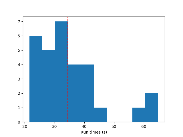
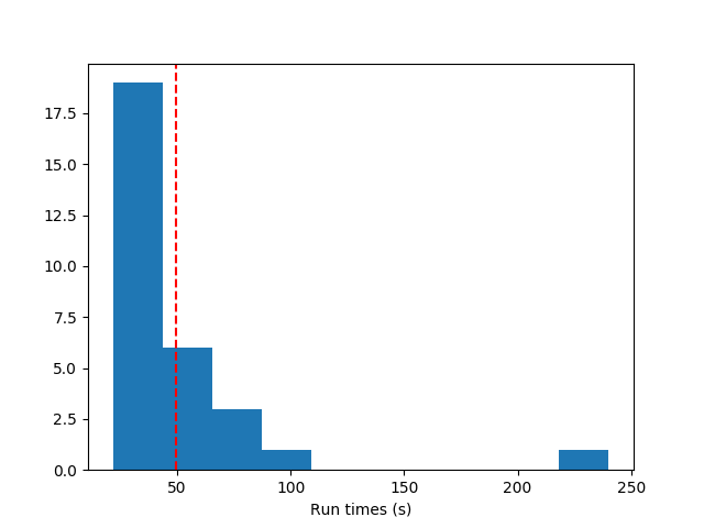
The one that adds more aggressively finishes faster.
Here's the progression of the node counts of the whole population for the more and less aggressive node additions:
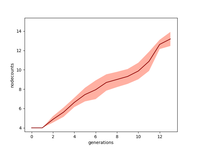
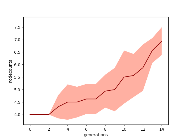
A bunch more for the more aggressive one, as you'd expect. Lastly, here are the final, best NN's produced by each of the runs above:
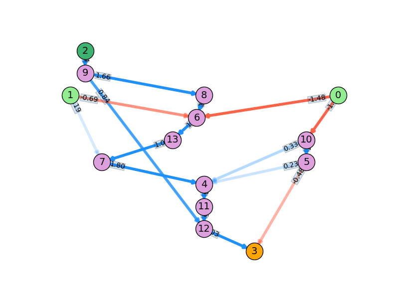
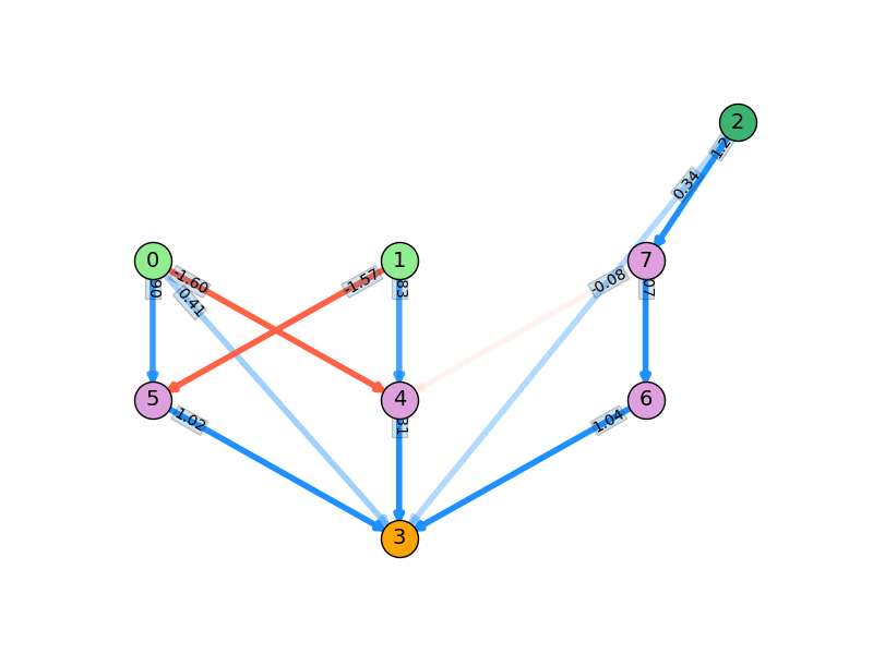
There's even redundancy with the simpler one, but the aggressive one is really inefficient.
If you want to be a little loose with analogies, I think this is similar to simulated annealing. If you included some regularization so that NN's paid a cost for being more complex, then this would correspond to them reaching a lower final energy state if you make them take longer to reach it. To make it a little more concrete, I might actually experiment with giving it something analogous simulated annealing's temperature: maybe I'll try making the add/remove mutation rate very high at first, and then slowly lower it over the generations.
This effect is especially important for the GD-free method, because there it has to figure out the magnitude of the weights too; it's possible that a NN already has the perfect topology but the weights just need a few more generations to mutate. This is reflected in the values of the probabilities I've seen used in the literature (for GD-free methods): $p_{add node} = 0.0005$, $p_{add weight} = 0.09$, $p_{change weight} = 0.98$, $p_{remove weight} = 0.05$. So you can see that it's almost always changing weights, but adding nodes/weights is a really rare thing.
On the other hand, for the GD method, I'm still a little confused. I definitely have evidence suggesting that the slower you make it change the topology, the simpler NN's you end up with. However, why exactly? If we assume (and I have good evidence for this) that it doesn't have the same problem the GD-free method does, with having a NN with correct topology but incorrect weights (because it seems to successfully train the weights quickly when it has the topology available), then why wouldn't you want to be adding as much as possible? A NN can only add nodes/weights, so if it does neither in a turn, it's kind of a wasted generation for it. One possible reason I can think of is that you probably do want to avoid adding both a weight and node in the same generation, because one of them alone may have solved it, but the other made it harder to.
What learning rate to use? How many training examples?
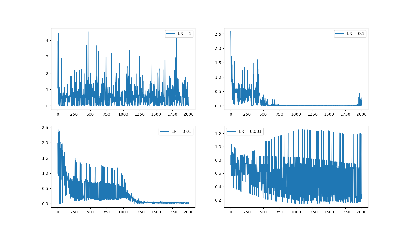
I used Pytorch's Adam optimizer to do GD on the weights. Adam is adaptive, but the initial learning rate (LR) you give it can still have a large effect (especially if you're doing such a small number of training samples). I tried a few initial LR's, testing it on a NN that I knew had the simplest working structure for a NAND gate:
Here's a single run of each, to give you an idea of what they look like:
But here's a more meaningful mean/spread over 20 runs each:
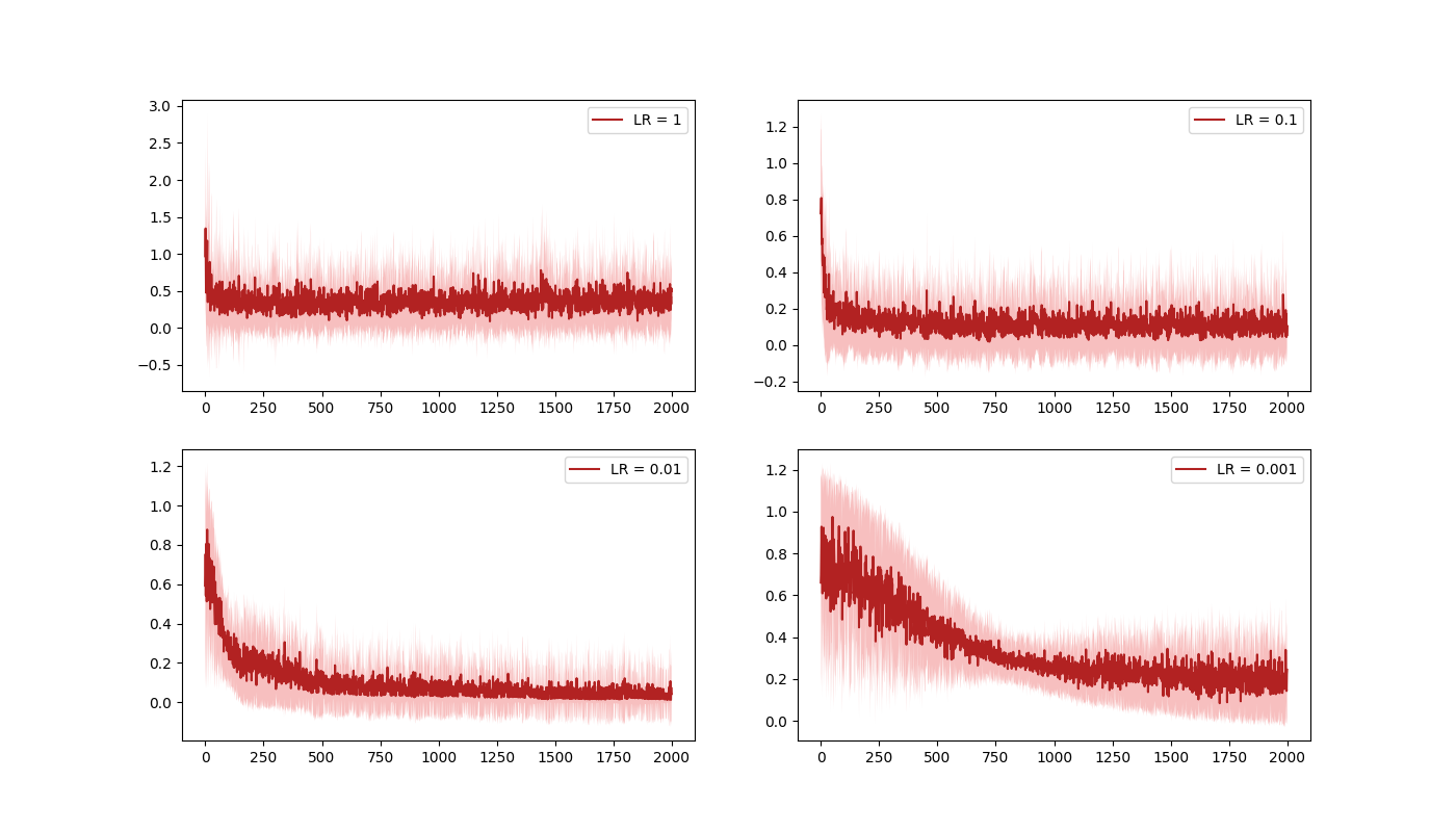
You can see that 0.1 and 0.01 both work pretty well. I went with 0.01 in the end because it seemed slightly better behaved, if sometimes a little slower.
How many training samples to use?
Obviously, using 300 samples to train a NN is atypically small. However, the runtime was a concern for me, and a large part of the cycles went to doing backprop during training, so I had to find a good balance between making sure the NN would get trained enough to actually improve once the topology was good enough but also not wasting a ton of unnecessary time on training (keep in mind that most NNs won't improve much at all with training because they just don't have the necessary topology).
You can get an idea of the scales in the figure above with the LR. There, it seems like you probably need 500-1000. I was using 300 to start with (for no real particular reason), so I tested it with 800 instead. However, I found it made it take a lot longer. To test the other direction, I tried 150 instead, which I also found to be longer. It seems lucky that what I started with was a decent choice, but it's plausible given the toy results above.
Should we reset the weights each generation?
One thing I was worried about was whether I should reinitialize (using roughly Xavier initialization) the weights before each training. Local minima are definitely a thing with NN training, so I was worried about the possibility of "training" the weights of a not-solved topology NN, and then when it finally gets a solved topology, being stuck in a local minima. However, this was apparently not the case, as reinitializing the weights before each episode made the GD method waaaaay worse. I was actually surprised by how much worse they were.
The code for this is here.