[latexpage]
So last time, I solved the egg drop puzzle in a few ways. One of them was using a recent learn, Markov Decision Processes (MDP). It worked, which got me really stoked about them, because it was such a cool new method to me.
However, it's kind of a baby process that's mostly used as a basis to learn about more advanced techniques. In that solution to the problem, I defined the reward matrix $R_{s,a}$ and the transition probability matrix $P_{a,s,s'}$, and then used them explicitly to iteratively solve for the value function v and the policy p. This works, but isn't very useful for the real world, because in practice you don't know $R$ and $P$, you just get to try stuff and learn the best strategy through experience. So the real challenge would be letting my program try a bunch of actual egg drops, and have it learn the value function and policy from them.
Here's how I implement this. If I'm solving for $N_{floors}$, I say I have 2 + 2*$N_{floors}$ states. s = 0 is the "solved" state, where you've determined the correct break floor. s = 1 is the "both eggs broken" state. States s = [2, 1+$N_{floors}$] are states where you have 1 egg, and are on floor f=(s-1). States s = [2+$N_{floors}$, 1+2*$N_{floors}$] are states where you have 2 eggs, and are on floor f=(s-$N_{floors}$-1). For actions, a=0 means dropping on the 1st floor, a=1 means dropping on the 2nd, etc. So Q, the action-value matrix, and E, the eligibility trace matrix, both using this ordering.
My code is broken up into two classes: EggdropAgent, and EggdropEnvironment. I like this because it really emphasizes that the agent is model free, in that it only gets to "sample" the environment, and doesn't know the background mechanics of it.
For a given episode, EggdropAgent will call EggdropEnvironment's generateEpisode() function, which will choose a "break floor", the floor the egg breaks if dropped from or above. Then, EggdropAgent will repeatedly call the environment's performAction(S,A) function, which will return R and S'. The agent will then get the next action A', and do the SARSA update.
I should also briefly mention what performAction is doing behind the scenes. It first determines e (eggs remaining) and f (floors remaining) from state s. Then, it determines if the egg breaks or not (i.e., (a+1) >= break floor). All rewards are -1 (representing one dropping of an egg, which we want to minimize the total number of), except for if you break an egg in a 1e state. Then, the reward is massively negative, -9000, because we really want the agent to avoid this (I'll talk more about this later). It then does some arithmetic to figure out how many floors you have left given whatever happened during that drop.
So, here's the agent code for learning a single episode:
def learnEpisode(self,starting_state=None):

    self.R_tot = 0

    #This will run one full episode with the environment, learning at each time step.
    self.time_step = 0
    self.state_history = []

    #Reset the eligibility trace matrix
    self.resetE()

    #Get the starting state (N floors, 2e) and put it in the history array.
    if starting_state is None:
        self.s = self.getTopFloorStartingState()
    else:
        self.s = starting_state

    self.state_history.append(self.s)

    self.a = self.getAction(self.s)

    #Generate the episode
    self.env.generateEpisode(self.getFloorsAndEggsRemainingFromState()[1])

    while True:

        if self.s==0:
            #print('in solved state, exiting!')
            return((0,self.R_tot))
            break
        if self.s==1:
            #print('in both eggs broken state, exiting!')
            return((1,self.R_tot))
            break

        #So above this line, you have the SA from SARS'A'.
        (self.R,self.s_next) = self.env.performAction(self.s,self.a)
        self.R_tot += self.R

        self.a_next = self.getAction(self.s_next)

        #Increment E and update Q, and then decay E
        self.incrementCurStateActionE()
        self.updateQ()
        self.decayE()

        #updating s and a
        (self.s,self.a) = (self.s_next,self.a_next)
        self.state_history.append(self.s)
Here are the important steps:
- Reset E (the eligibilities of the states for the episode)
- Choose the starting state (the default is the top floor, but I add the option (see below why) to start at any state)
- Get the action from that state (greedily or $\epsilon$-greedily)
- Generate the episode from self.env (the environment)
- Repeatedly:
- If in a terminal state (s=0 or s=1), return the ending state and total reward
- if not, performAction(S,A), get R,S'
- get next action A'
- update E and Q
- set S,A to be S',A', moving the "current state" forward
Results! How does it do?
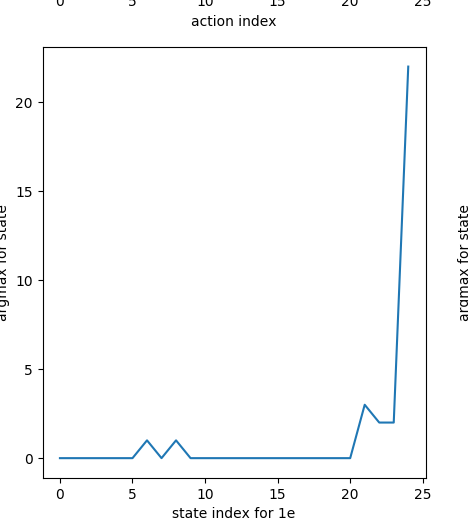
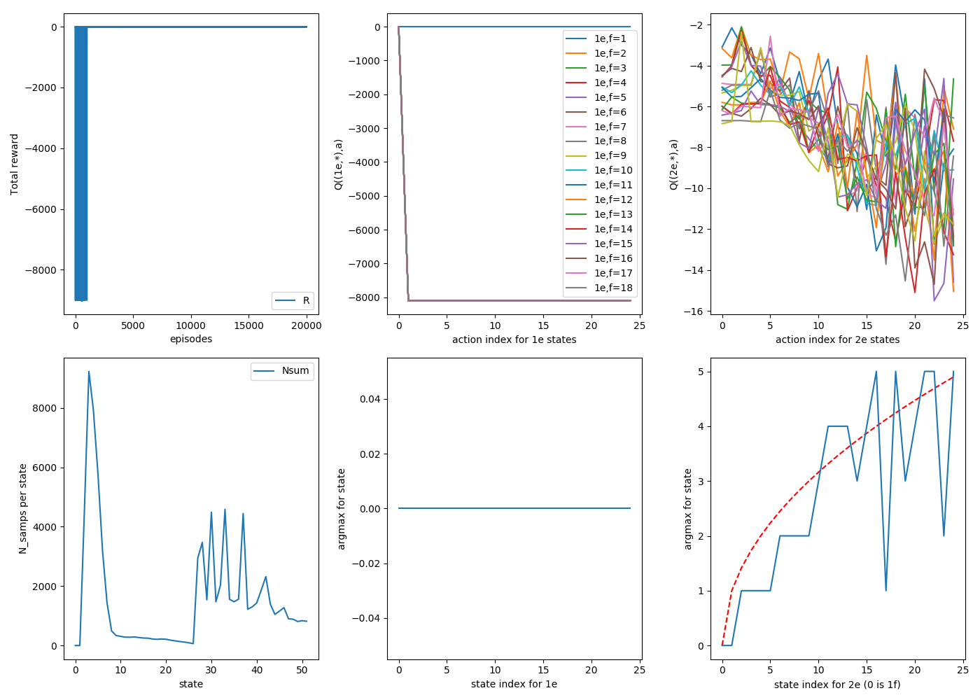
Not great, at first. Let's first just mention what we'd like to see, if it was working nicely. We'd like to be able to plot the argmax over all actions for each state, $\textrm{argmax}_a(Q(s,a))$, which would tell us the best action to take in each state. If you look at my last post, this would mean taking action 0 (i.e., dropping on floor 1) for all the 1e states, and action int(sqrt(f)) for all 2e states with f floors remaining. When you have 1 egg left, you have to scan from the bottom, meaning dropping on floor 1 each time until you have 1 floor left. If you have 2 eggs, sqrt(f) gives you the best balance of skipping floors and minimizing the risk of breaking.
So, here's what we get for $\epsilon$ = 0.05, decaying by 0.999 each episode, $\gamma$ = $\lambda$ = 0.99, $N_{floors}$ = 25, 20000 episodes.
This is the argmax of Q(S,A) for each state, for 1e and 2e separately:
1e:
2e:
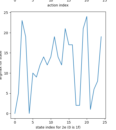
Ooooof. The 1e states have mostly settled to the right value (a=0), but the 2e states are nowhere near sqrt(f).
Here's where I started getting into some real nitty gritty and having a good learn.
The first thing to notice is that luck plays an inconveniently large role in this problem. For example: let's say you're in state (1e, 25f), and the break floor happens to be 23. Usually, dropping on floor 23 would be a terrible move, but in this case, it actually ends up letting you skip a ton of floors, giving a good reward for that action if the episode finishes. Of course, this is very uncharacteristic for that (s,a) combo, but it will remain there until it tries it again and corrects it once it (probably) gives a more representative reward. However, that could be a while, especially for relatively rare states like (1e, 25f).
Similarly, but more commonly, it can take a while for the "skip vs risk" balance of the optimal sqrt strategy to manifest. That is, even doing the actual optimal strategy of sqrt(f) for 2e, it's still going to break your first egg sqrt(f)/f = 1/sqrt(f) fraction of the time, making you scan a ton. So when the agent has limited statistics to learn from, it's going to have a pretty hard time seeing the benefit of the optimal sqrt strategy.
Here's what I figured out after a lot of thinkin' and tinkerin'.
The role of $\lambda$
TD($\lambda$) is a really cool technique, but for this problem, I you think you really don't want a $\lambda$ term at all. The role of $\lambda$ is to let all the rewards from an episode directly change the Q values of the earlier states of the episode that gave rise to the later states, via the eligibility traces. While this lets your states update with information and often makes them more robust to being too near or far sighted, I think for this problem, you can't allow the results from actions taken in much later states to affect earlier ones directly.
I think it might depend on how you set up the problem, but I wanted the "breaking both eggs" reward to be so hugely negative that it enforces a "you absolutely can't risk this happening", and I think this should be fine, if the parameters are chosen correctly. Here's an example of why. Pretend the agent starts in the (2e, 25f) state and drops on 5 (the best move!). The egg breaks, and now it's in the (1e, 20f) state. It drops it on 10 (pretend it's still dropping with some $\epsilon$ randomness) and it breaks again, getting the huge negative reward. Now, if $\lambda$ isn't 0, it's going to pass this massive negative reward back to the previous state-action pairs like Q((2e,25f),5), punishing them! The negative is so large that in the (2e, 25f) state, drop=5 will probably never get selected again.
So I think you really don't want any $\lambda$ for this problem, partly because of the huge negative reward and the large luck factor. I'm not sure, but you could probably set that negative R to be small enough (magnitude) that even if a state got screwed early by it, it could still be overcome by lots of subsequent good episodes, but it also has to be large enough that it doesn't become a "shortcut" for the agent! For example, for some value of R, it would be worth it for the agent to drop on an aggressively high floor always, since the punishment for breaking both eggs might be outweighed by the floors it would get to skip the times it doesn't.
We probably don't need epsilon greedy for this either
It turns out that $\epsilon$ greedy is actually a pretty bad policy for this problem, I think. As mentioned above, the 2e states really depend on the 1e states being relatively accurate and behaving correctly. In addition, the reward for breaking both eggs is so hefty, compared to the multiples of -1 that you're (ideally/typically) fighting to minimize, that getting unlucky and breaking both eggs due to the $\epsilon$-randomness can screw the Q for some (s,a) up for a long time.
Even if you have $\lambda$ = 0, $\epsilon$ greedy can still mess things up. For example, early on, each 1e state will try lots of actions (because after it tries drop=1, that will necessarily have a negative score, and then the argmax after that will be drop=2, etc). Some of these will definitely cause the last egg to break, giving that Q(S,A) a huge negative, even if that's not passed back to the earlier 2e state then. In a later episode, when updating SARSA, if the getAction() function was choosing greedily, it would never choose that 1e action that got the huge negative, and thus it wouldn't affect other state-action pairs. However, with epsilon greedy, it sometimes will, again allowing a bad state-action to ruin other ones.
Therefore, I think you don't really want $\epsilon$ greedy for this problem. The risks are too large, and I think in this problem it will actually naturally get its way out of local optima, given enough time.
So, how does it do with $\lambda$ = 0, $\epsilon$ = 0?
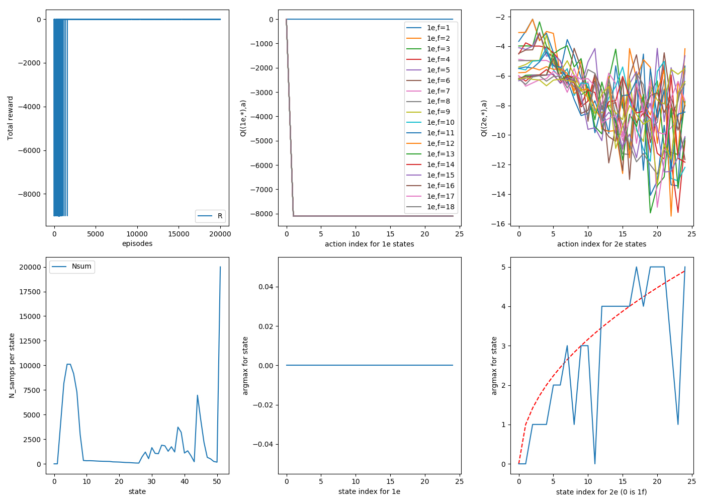
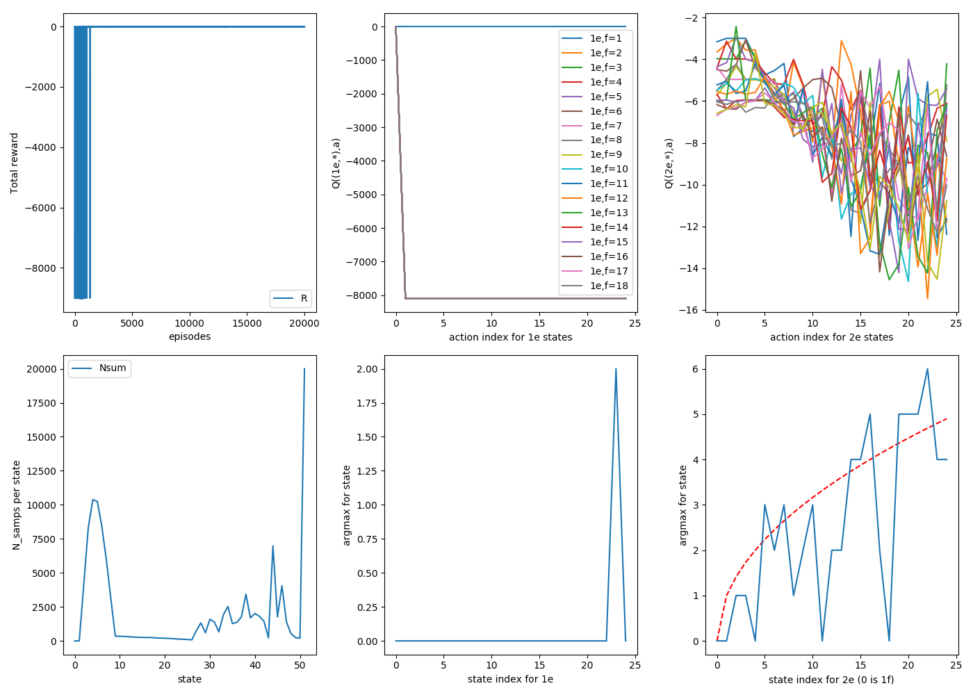
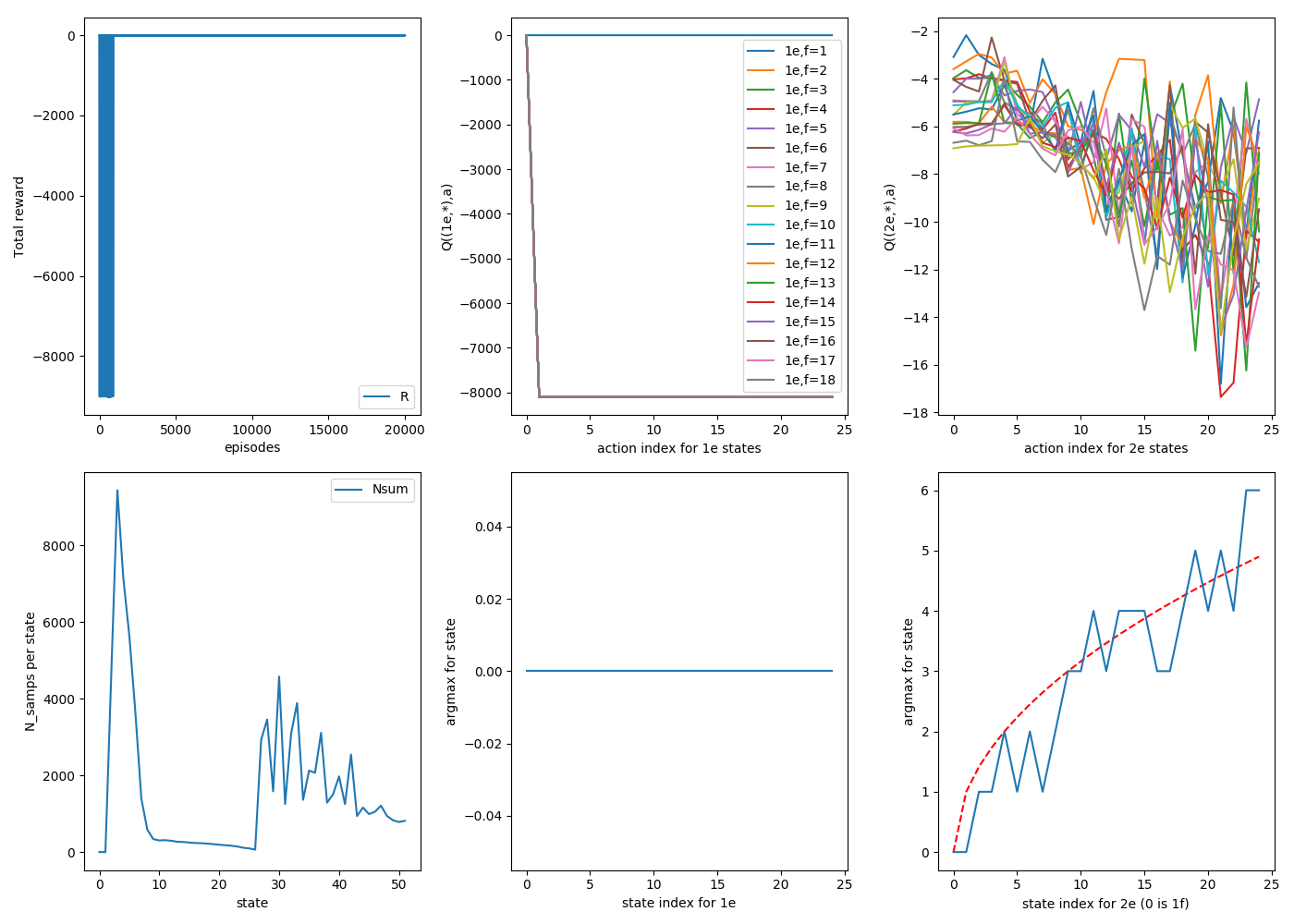
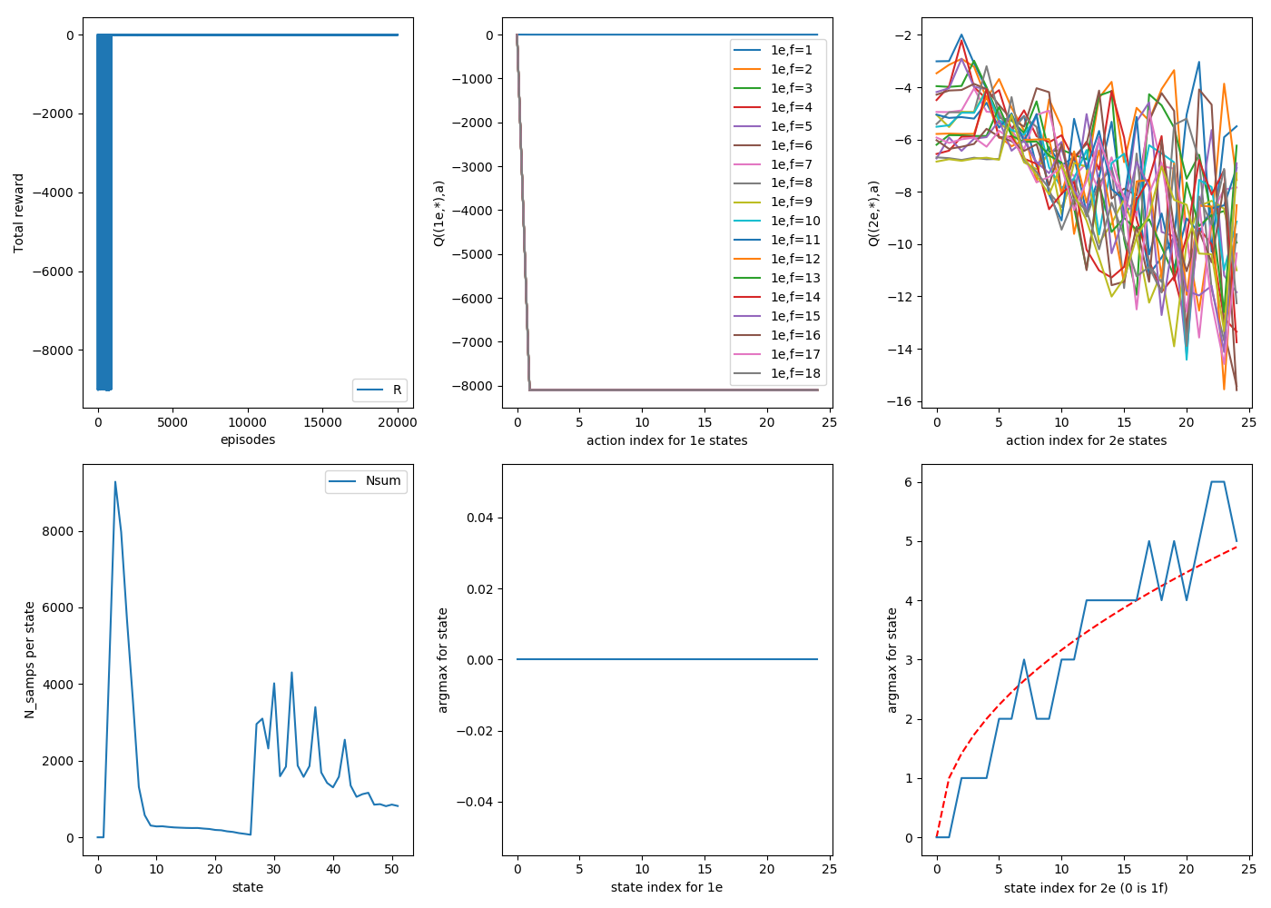
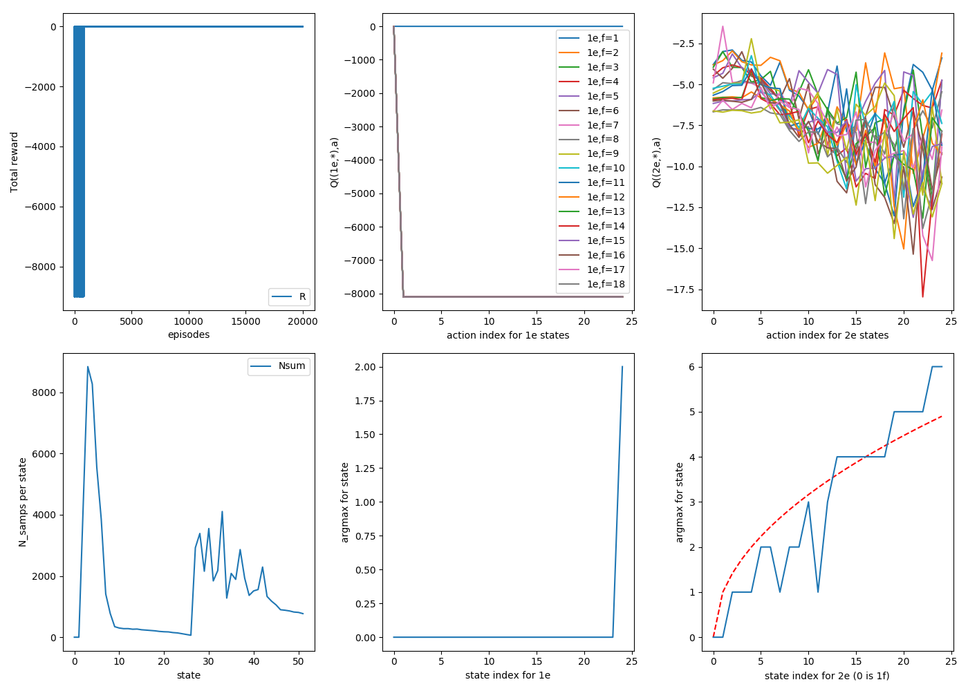
Here are three consecutive random runs, with 20,000 episodes each. For now on in this post, assume that $\gamma$ = 1 unless otherwise stated. For these runs, $\alpha$ = 0.9, and each episode starts by dropping from the top floor ($N_{floor}$ = 25).
1
2
3
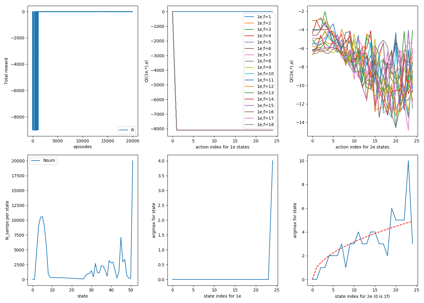
The "goal" is in the bottom right plot, where the sqrt of the floor state is plotted in red, which is what we'd like the argmax curve to look like. You can see that for all three, they definitely track it, though to varying tightness; there are definitely some jagged ones off of it.
For good measure, here's the same thing, but with 200,000 episodes:

It definitely looks smoother. There are a few things to point out. First, looking at the bottom middle plots, you can see for all runs, they've figured out the correct strategy for 1e states perfectly: always drop on 1. You can see the actual Q values for these states as a function of action: all actions besides a=0 (drop 1) eventually get stung by breaking the second egg, and correctly never do them again.
Another thing to notice is the distribution of samples per state, the bottom left plot. The 1e states (s = [2,1+$N_{floors}$]) are very lopsided. This is because, as the 2e states begin to figure out the strategy, they're rarely dropping it from high floors, meaning that it rarely ends up in a high f, 1e state, so they just don't get sampled much.
That's fine, because those ones quickly find their correct values anyway, but if you look at the 2e states of that plot (s = [2+$N_{floors}$, 2*$N_{floors}$+1]) , you'll see a weird, jagged, semi regular set of spikes. These are because, as it forms the 2e strategies, these will also determine what states tend to get sampled. For example, for (2e, 25f), if it determines that dropping on floor 6 is the best strategy, it will either not break and now be at (2e,19f), or break and be at (2e, 6f), but either way it won't get to (2e, 21f). If you look closely, I think the ones with wonky argmax values are usually ones that haven't been sampled much.
I can actually do a little fix for this, which is choosing to start the episode by dropping with 2e on any floor. This will sample the 2e floors more evenly. I don't think it's "cheating" because we could just run for longer, and it's really only fixing states that aren't visited much anyway, making diagnosing the real issues easier.
Here's the same thing, but starting randomly on any floor. Three 20,000 episode runs:
1
2
3
As you can see, generally a smoother argmax and a more even distribution of samples. This is what I'll do for the rest of the post.
The learning rate
So far I've been using a learning rate $\alpha$ = 0.9. This comes into play when you've calculated the TD error in the SARSA algorithm and you're using it to update the Q values. In code:
def TDerror(self):
    return(self.R + self.gamma*self.Q[self.s_next,self.a_next-1] - self.Q[self.s,self.a-1])

def updateQ(self):
    self.Q += self.alpha*self.TDerror()*self.E
    self.updateN() #Just increases the sample count for this (S,A) pair.
An $\alpha$ of 0.9 is pretty aggressive, in that it will try increasing Q(s,a) by the difference between what that iteration thinks Q(s,a) should be and Q(s,a)'s current value. This is fine if the thing its aiming for (R + Q(S',A'), the "TD target") is correct or stationary, but in our case, even when you're making the optimal choice, say, drop=5 for (2e,25f), 20% of the time you're going to break that egg and get the relevant (R + Q(S',A')) for that, and 80% of the time you'll get the (R + Q(S',A')) based on the other outcome. Then, if you're just adding $\alpha$ times the error each time, you could imagine Q(S,A) oscillating around the "correct" value wildly. For this problem especially, you want Q(S,A) to reflect the average value for taking action A, and having a large $\alpha$ might make the value of Q(S,A) more just "listen to the last guy he talked to".
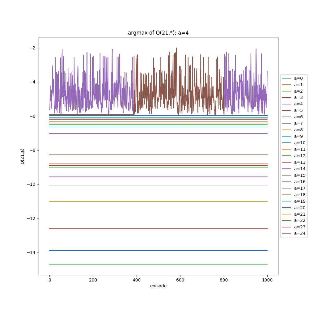
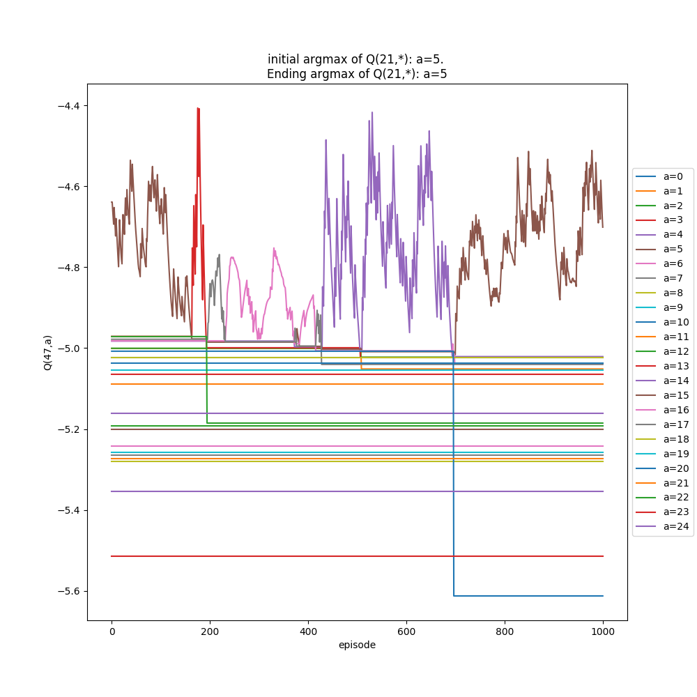
To show this more explicitly, I made a function inspectState(S) that I can call after running many episodes (i.e., what you've seen so far are the plots of that) that will run more episodes all starting from the single state S, letting it learn more by dropping from only that state, and plot the Q(S,A) values over those "extra" iterations. I ran the above ($\alpha$ = 0.9, 20,000 initial episodes, starting from random floors), and then chose f=22 to "inspect" for 1000 more episodes. Here it is:
You can see the wonky argmax values for high f, 2e states, in the bottom right again. But if you look at the plot below, you'll see that the argmax of (2e,22f) is actually switching between two values over time!
I tried a couple things here, and to be honest I'm not sure what the takeaway is. My first guess was that maybe $\alpha$ is too high, so I tried to vary it to see how it affected the error. For this problem, I'm calling the error the Mean Squared Error between the argmax of the 2e states and the square root of the floor number for each of those states, since that seems like a good metric. I varied $\alpha$ from 0.05 to 1.4, for each value of $\alpha$, did 5 runs so I could get a bit of the mean/stdev, and I repeated the whole experiment for three different numbers of episodes (2000,20000,200000). Here are the results:
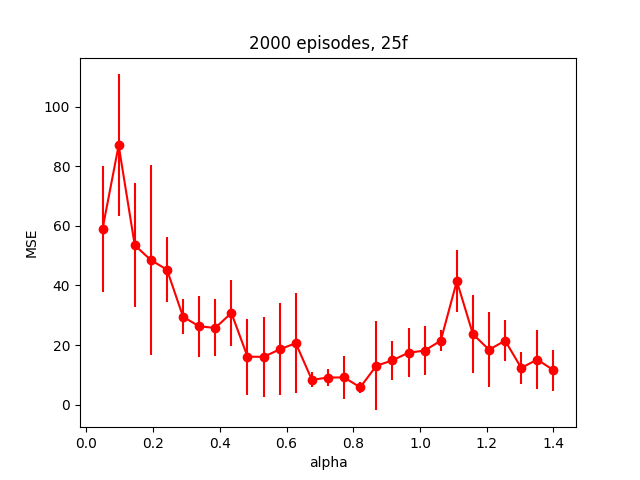
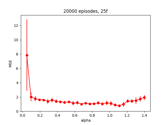
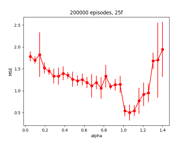
So it seems like it's probably just not converging much at all for the runs with 2,000 episodes, to the point where all $\alpha$ values suck. It seems like the runs with 20,000 episodes are all pretty similar for $\alpha$ > 0.1 (MSE really only varying from about 1-2). The runs with 200,000 episodes look crazier, but if you look at the actual MSE range, it's about the same as the 20,000 episodes one. Additionally, it appears to have a minimum at alpha ~ 1.1, same as the 20,000 one.
So this is surprising to me. First, I thought my $\alpha$ was probably too big at 0.9, when in fact that's probably fine and maybe even too small. The other thing is that it just doesn't seem to have much of an effect. I wonder if this is because I've simplified it so much by making $\epsilon$ and $\lambda$ both be 0?
I tried a few other things. The first is updating Q(S,A) less as (S,A) gets more samples. This just means replacing the updateQ() line above with:
def updateQ(self):
    self.Q += self.TDerror()*np.multiply(1.0/(self.N_samps+1.0),self.E)
    self.updateN()
Doing this with [2000,20000,200000] episode runs, 5 runs of each, gives the following:
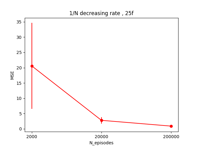
It's hard to see the scale for the 200,000 point, but its value is 0.9, which is about the same as for the best alphas in the 200,000 plots above. The avg of the 20,000 episode point runs is 2.8, which is actually somewhat worse than all the values of $\alpha$ for the 20,000 episodes $\alpha$ runs above.
I tried the same thing, but using 1/sqrt($N_{samps}$) instead, so it decreases more slowly. This gave:
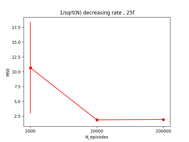
So pretty much solidly worse. In fact, the 200,000 episode set is actually worse than the 20,000 one...
Lastly, I tried another averaging method. If you look at the "decreasing by 1/$N_{samps}$" methods above, it means that the earlier values submitted to Q(S,A) count more towards changing it than later values, because each subsequent value that's getting added to Q is getting a 1/N (or 1/sqrt(N)) factor. So that's not really a true average, and I though it might be possible that early, bad values that contributed to Q might affect it for way longer than desirable, since the later values that could "fix" it count for less. So what would make it a true average is to do Q <= (Q*N + $TD_{error}$)/(N+1), like so:
def updateQ(self):
    self.Q = np.multiply((self.N_samps*self.Q + self.TDerror()*self.E),1.0/(self.N_samps+1.0))
    self.updateN()
How did this do?
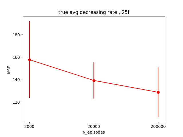
Ooof. That is terrible. Honestly, I'm not sure why, either. This "true average" method should actually become the 1/$N_{samps}$ method for large N! So that implies that the changes from early (S,A) are actually really important here, because that's the difference between this method and the 1/N one. I'll have to think about this more.
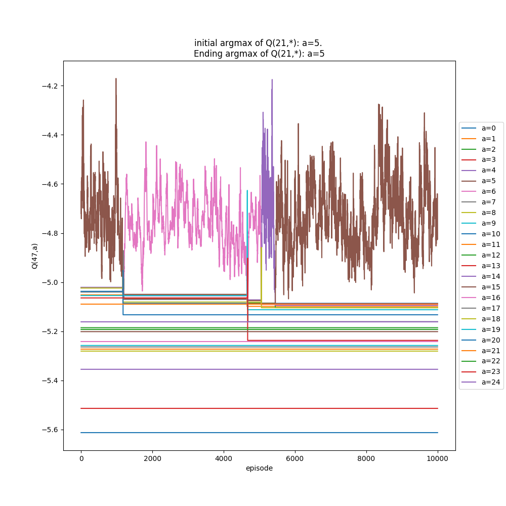
I'll briefly show two more things. The first is what the "inspect" plots look for two different alphas, 0.1 and 1.1. Remember from above, it seems like $\alpha$ = 1.1 should be the better choice. For each of these, I first run the whole thing with 200,000 episodes, then inspect state (2e, 22f) (randomly chosen high floor, so more likely to change its state with more samples). I inspect that state for 1,000 extra drops (starting from it), and then 10,000 immediately following, to see the short and long term effects if there are any.
$\alpha$ = 1.1:
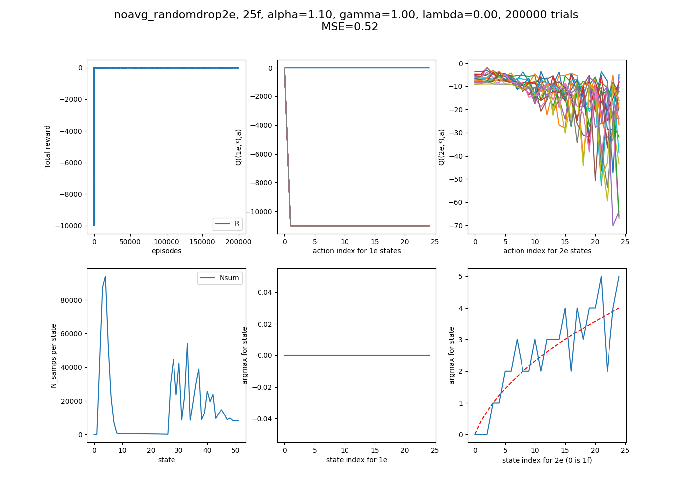
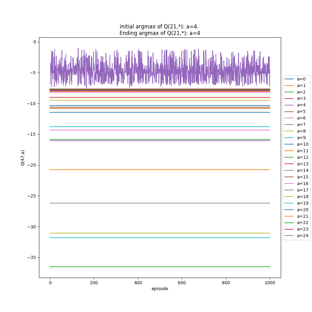
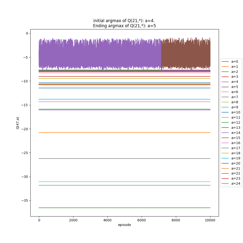
You can see that the argmax tends to be more stable, but also has a pretty big range (~5). It only switches once in the extended "inspection".
$\alpha$ = 0.1:
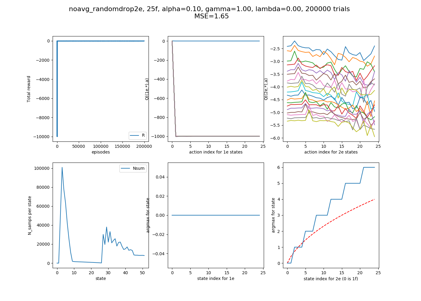
A few things to notice. First, the MSE is worse, as expected. The 2e argmaxes actually look "better behaved", i.e., monotonic, but they diverge too much for high states, giving the high MSE. This is probably because the lower states (that higher states depend on) are correctly getting figured out which ones are the best choice, but they can be known to be the best action and still have an inaccurate Q value. You can also see in the upper right plot, the plot of Q(S,A) vs A (with the different curves being for different S's) that the argmaxes (little peaks) are a lot more pronounced. This is because the bad ones aren't as severely punished because of the small $\alpha$ value. Compare it to the $\alpha$ = 1.1 one above, where the non optimal Q(S,A) values are much more negative. Similarly, the same plots but for the 1e states (the top middle plot) goes down to -10000 for $\alpha$ = 1.1, but for $\alpha$ = 0.1, they don't get as much of the huge negative, meaning they're only 1,000.
Next, looking at the inspection plots, you can see that 1) they switch a lot more, and 2) the range they oscillate in is a lot smaller (~0.8). I was initially hoping that the smaller $\alpha$ would mean that the argmax for a state is actually more stable, because unlucky events wouldn't mess it up as much, but I think the flip side of that coin is that the non optimal actions aren't punished as much, meaning they have a bigger chance of "bouncing back" after some unlucky events as well.
Lastly, let's just look at one example with more floors. I've been using 25 floors because it was big enough that hopefully we could see the sqrt behavior if it was doing it, but also small enough that a given number of episodes could let it converge. However, let's run it at 100 floors for good measure, to really make sure it's doing the right thing.
200,000 episodes:
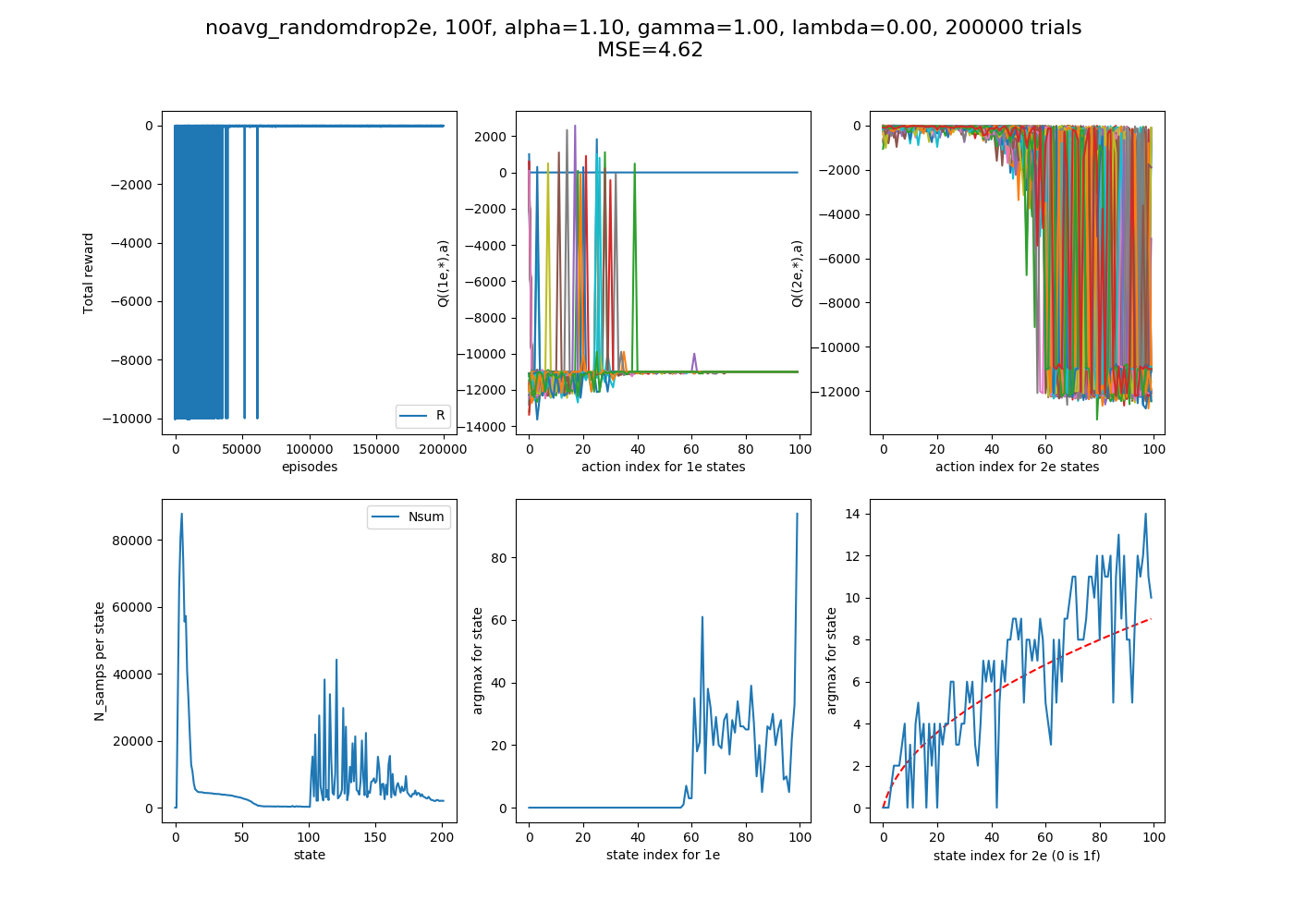
Pretty messy, and you can see that not even all the 1e states have converged (probably because some haven't even gotten to try all their actions, so if the action hasn't been tried, the Q(S,A) is the starting value of 0, bigger than negatives that accrue from actually trying actions). I thought that trying 2,000,000 episodes might improve it, but...
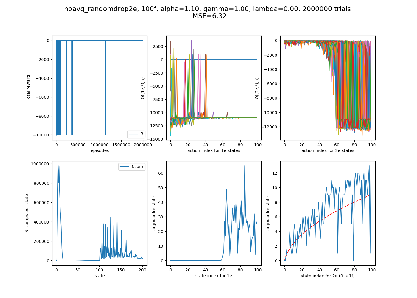
I'm not sure what to take away. It's possible that the randomness of this could cause this stuff, since there are a lot of states, but it's still confusing. Still, this should show that it's definitely finding the right path, even if it takes a while.
Anyway, that's all for now. This was a fun project that started pretty randomly but got me on the RL path. I still have a lot of questions about the problem and RL in general, though: Is this a unique problem, with its dire consequence for breaking two eggs? Does a consequence like that really mean that you should avoid use of $\lambda$ and $\epsilon$?
Right now, my Q(S,A) is initialized to all 0's. Since each episode always gives a negative reward, that means that, in a state, it will actually keep trying new actions until it has tried them all. In a way that seems good, because it's automatically doing exploration, but it also seems like it's different in nature from what I feel like I see in some problems, where it's more of a positive feedback loop (i.e., the agent tries an action, gets a positive reward, now that action is even moreso the argmax, and it keeps trying it).
Another thing I might do one day is, I'm afraid I may have put too much of a "model" into the problem. That is, when I do performAction(S,A), it automatically returns you to the "subproblem" (for example, if you have 100 floors left and drop on 34 and it doesn't break, it then puts you in the state with floor 66). This is true, but maybe it's giving insight to the model, whereas the most model free agent could figure that stuff out on their own?