[latexpage]
Simulated Annealing (SA) is a very basic, yet very useful optimization technique. In principle, it's a modification of what's sometimes called a "hill climbing" algorithm.
Let's look at a practical example to explain what hill climbing is, and what SA addresses. Imagine you're in a 1-dimensional landscape and you want to get to the highest possible point. Further, a crazed optimization expert has blindfolded you so you can't see anything; all you can do is randomly try to go either left or right, by tapping your foot to feel if a step in that direction is higher than where you're currently standing. If it is, you take that step, and repeat.
And hey, it works pretty well!
You reach the highest point, and the waiting optimization expert reluctantly takes off your blindfold, muttering something about "stupid convex functions".
But maybe you see the limits of this search method. This time, you're plopped down in another landscape, and the sociopathic expert has done some hefty landscaping. You try your method again, and...
you're stuck in a Sisyphean optimization hell.
So, what can you do? Even though there was a higher spot than where you finished, you couldn't get to it because you've chosen to only take steps that are immediately up from where you started. In your desperation, you decide to be a little more adventurous, and still always take a step if it would lead you up, but with some probability, take a step that goes down:
Free again! You can see the dot wobble a little at the second little valley, where it has to get lucky several times in a row to overcome it.
So this is the basic idea: always accept a better solution offered, but also sometimes accept a worse one. The classic way of determining that "sometimes" is by calling your current height $E$, the height you're considering going to $E_{new}$, choosing a "temperature" $T$, and calculating:
$$p = e^{\frac{E_{new} - E}{T}}$$
which represents the probability that you'll take a step that takes you from $E$ to $E_{new}$. So for $E_{new} > E$, $p > 1$, for which we just take the step (so if you want to be precise, $p = \textrm{min}(e^{\frac{E_{new} - E}{T}}, 1)$), but if $E_{new} < E$, we only take the step with probability $p < 1$.
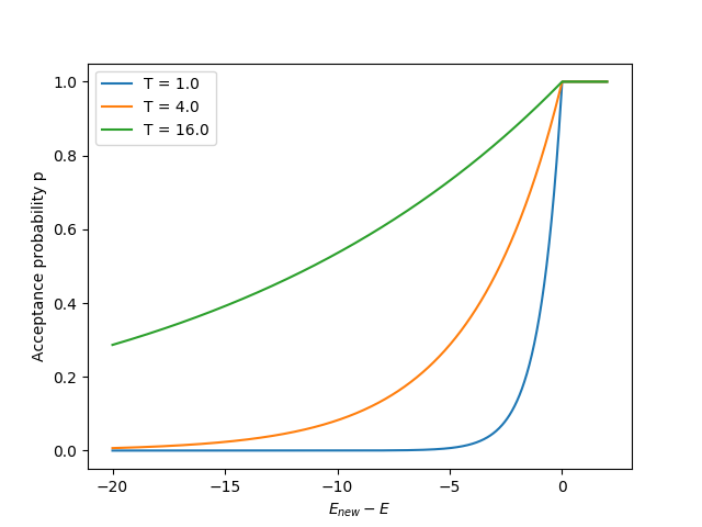
Note two significant aspects of this form: 1) it allows you to take worse steps, but the worse the step, the less likely you'll take that step, and 2) $T$ acts as a multiplier to this effect; if $T \gg 1$, then $p \sim e^0 = 1$, meaning it will accept anything, even if $E_{new}$ is much worse. Conversely, if $T \ll 1$, it makes any $E_{new} - E$ difference huge, and therefore it'll only accept steps that are better... which is exactly what we were doing originally! As you'll see below, this is really important.
Here's a plot of $p$ for a few values of $T$, as a function of $E_{new} - E$:

We'll come back to this, but here's an example you can try out yourself to get a feel for it. In a previous article, I solved the Brachistochrone problem with a genetic algorithm. Briefly, the Brachistochrone is the curve between two points such that if you released a bead from the higher point and it was constrained to that curve, with force of gravity on it, it would take the shortest time to reach the lower point (see the article for details).
Here's an interactive example of it. Try dragging the points around to make a bad initial solution, and then hit Run to try and solve it!
You can also vary the temperature, mean amount of change, and height difference, and hit Run again to do more iterations with the same curve. You can see that if you use a high $T$, it accepts all sorts of solutions, and if you use a low $T$, it only improves, but often pretty slowly.
So this method works pretty well for these two scenarios, but it still isn't the whole story. To see why, let's go back to the hill climbing story and make it slightly more complex. While before you took a step of constant size to the left or right, pretend now that not only is your direction random, the size of the step is too; your step size probability is a Gaussian distribution with a mean of 5.0.
And again, the sneaky expert has thrown you a curveball: they've made the hill textured as hell, with lots of local maxima. Now, let's see what happens when you try it with the acceptance probability from above, $p$, and a low $T$ of 0.1 (causing you to mostly only take improving steps):
You never get very far, because you'd have to leave the local maximum found very early.
You could try using a large T instead, so you won't get stuck up there. Here it is with $T = 80$:
Well... you explore more and get a better overall score, so that's good! ...but you also never more thoroughly explore the area around the true maximum, because you're so willing to accept anything. So the max height you reach is closer to, but not the true maximum.
So you can probably see the problem and a potential solution. You need a large $T$ at the beginning to accept worse steps to get out of local maxima, but you need a small temperature at the end to only accept better probabilities. This is what simulated annealing does: start with a high $T$ and slowly lower it, so the willingness to accept worse steps, $p$, goes down over time. You can decrease it in all sorts of ways, but a simple one is doing: $T_{i+1} = \lambda T_i$, where you can choose some $\lambda < 1$ to make $T$ start at some value and decrease to ~0 by the time you want to be done.
Let's try the nasty problem again with this! Here it is with $T_{init} = 80$, and $\lambda = (0.01)^{1/1600}$, because I'm doing 1600 iterations:
Ta da! You're the insane optimization expert now. And the cycle continues...
"Why is it called 'simulated annealing' though?", I hear you not asking. It's actually inspired by a phenomenon from physics. It actually comes from annealing in metallurgy, but I'm going to explain it in a very similar scenario: the Ising Model (IM). In two dimensions, the IM models a grid of atomic spins, which (here) can only have two values: up or down. When two neighboring spins are aligned in the same direction, their energy is lower, and vice versa.
Higher (undesirable) energy state:

Lower (desirable) energy state:

It's the same idea in 2D, but now you add up the energies for each pair in both dimensions (just counting its neighbors immediately up and down, left and right):

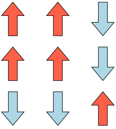
The IM evolves by spins being offered (randomly, one at a time) the chance to flip their direction, with the same probability of acceptance as above! For example, if the bottom center spin was offered to flip from blue/down to red/up, it would now align with two of its three neighbors in that new state, which would be more energetically favorable, so it would accept, and flip. Give it a try on a small example!
Here, instead of controlling T itself, you can control the decay rate lambda. Hit run to run for longer, or reset to go to a new random configuration and the initial temperature.
This illustrates the mechanism, but this example is too small to see the really cool stuff, because it's almost entirely boundary. Let's try with a bigger one!
Like before, a very high $T$ never settles to a low energy, and a low $T$ settles, but to a sub-optimal point. You can see a characteristic of a lower energy state: because spins aligned have lower energy, and larger clusters of spins in the same direction have smaller boundaries compared to their size, the average cluster size increases for lower energy. So, try different temperature decay rates, and see how they affect the final cluster sizes!
Welp, that's all for now! There's a lot more to simulated annealing I didn't even touch on, like restarts, tabu search, and other stuff... so maybe in a future post! Please let me know if you have any questions or feedback.