[latexpage]
After I trained an agent to play "puckworld" using Q-learning, I thought "hey, maybe I should make a real robot that learns this. It can't be that hard, right?"
Hooooooooo boy. I did not appreciate how much harder problems in the physical world can be. Examples of amateurs doing Reinforcement Learning (RL) projects are all over the place on the internet, and robotics are certainly touted as one of the main applications for RL, but in my experience, I've only found a few examples of someone actually using RL to train a robot. Here's a (very abridged!) overview of my adventure getting a robot to learn to play a game called puckworld.
First, simulation
The first thing I wanted to verify was whether a slightly different version of the game could be solved with the same neural network (NN) architecture. When I simulated it before, I used a NN with 4 state inputs $(x, y, x_t, y_t)$ (where $(x, y)$ is the agent position and $(x_t, y_t)$ is the position of the current target), 4 action outputs (up, down, left, right), and a single hidden layer (with varying numbers of neurons; I found relatively similar behavior over the range of 10-200 neurons).
However, I planned on using a robot of this style, which meant that its actions would instead be (forward, backward, CCW turn CW turn). The state vector is a little more complicated, but for now let's assume it's $(x, y, \theta, x_t, y_t)$ ($\theta$ is the angle, where $\theta = 0$ is pointing to the right, ranging from $-\pi$ to $\pi$, CCW).
It's not that I had doubts about whether it could be simulated at all (it's pretty simple either way), but it wasn't immediately clear to me whether the same simple NN architecture that worked for the original "cartesian" version would work here. I wanted to check this because while I could easily imagine the ideal NN that would work for the original puckworld, the radial one is inherently nonlinear and I couldn't immediately say what kind of operations it would need to do to determine the optimal action.
So, I wrote up a PuckworldAgent_robot class and gave it a spin! Here's the average reward curve and how it performs after learning:
(the animations don't autoplay in all browsers, so you may have to click on it.)
It also has no velocity state term (whereas the original PuckworldAgentdid), to reflect the fact that the real robot will never "drift" if the motors aren't driving. I also tested a few other little variants, like making the turns rotate it $90^\circ$ plus some zero centered Gaussian randomness, which it was all pretty robust to.
Anyway, that confirmed that I could probably do it without having to explore different architectures or learning methods!
The robot agent
For the robot itself, I went for the dinkiest robot kit I could find on Amazon:
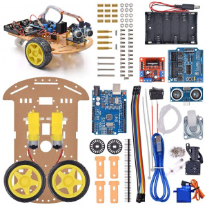
For about 20 bucks, it comes with a bunch of stuff. I mostly wanted it for the chassis, motors, driver, and wheels. The robot went through many iterations, but I'll talk about those details in a future post and just briefly cover the final version here.
The robot body is pretty large, but it actually ended up being pretty cramped with all the stuff I needed on it! Here's what it had by the end.
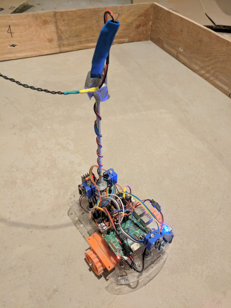
The Raspberry Pi that controlled it:
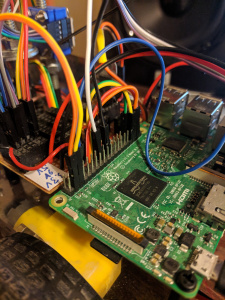
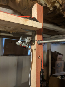
I also used a MPU9250 IMU module to find the current angle (from its compass). To get distance data, I used three VL53L0X TOF modules (that I designed and 3D printed the mount for in this post):
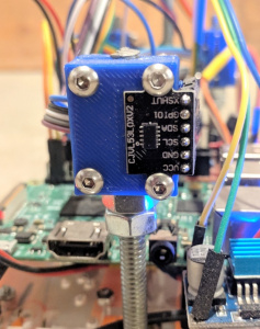
These are some pretty amazing modules! More on them later.
Lastly, all these had to actually be put together and powered, which I did on a separate little circuit board:
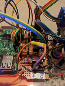
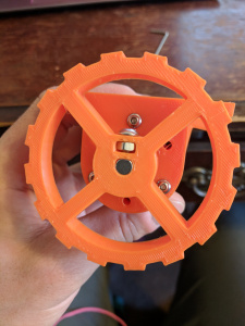
It might seem like a bit of a rats nest, but it makes it pretty easy to hub all the I2C devices together and power them. In addition, the motors run on 12V, the RPi on 5V, and the peripherals on 3.3V, so that took a few regulators. I also eventually got beefier motors, so I 3D printed wheels and mounts for them:
It would've been nice to just use a battery pack to power it, but with the current draw of the motors and a chuggin' RPi, any battery pack wouldn't have lasted too long. So it was actually wired the whole time, so that it would be able to run for days on end. To do this and and allow the robot to turn infinitely and move around, I used a slip ring and had the power cords mounted on a 1/4" rod about 8" above the robot (you can see in the first pic, where I used a bit of heat shrink to make it so it would both hold it up when there was slack so it wouldn't get tangled, but allow it to pull a bit when it's farther away from the center).
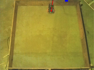
The environment
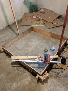
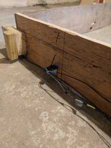
I wanted a little arena to enclose the robot just like the simulation. I used a few sheets of scrap plywood I found around my neighborhood and put them together with nubs of 2x4's in my basement:
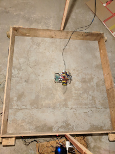
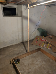
The frame at the top was to hold the slip ring and the camera for another Raspberry Pi (so I could monitor/control/calibrate it from my bedroom upstairs):
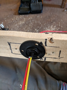
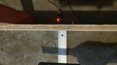
Lastly, for the actual targets, I used some IR sensors. I drilled holes in the side of the arena and mounted them. So there were 8 targets in total around the perimeter of the arena:
They have an IR emitter and sensor at the front and sense when something reflects enough of the emitted IR to the sensor. They also have a sensitivity screw that lets you control the "trigger range" from about 1-12".
They're real cheap (~a buck a piece) and not bad when they work... but they don't work for long. To be honest, they were kind of hell and I ended up having to replace at least one daily because they would just stop working.
The IR sensors went to an ESP8266 (kind of an Arduino that has built in WiFi support). The ESP connects to an MQTT server over my WiFi and broadcasts a json dict of the current state of which sensors are triggered, which the robot reads every iteration to see if it has triggered any.
The program
There were a million moving parts and details, but I'll just mention the main pieces here. I have an Agent class that does the actual Q-learning, saves the experiences, has the Q-network, etc. I wrote about how Agent does Q-learning here, so check it out if you're curious. It's basically standard Q-learning, using a NN with one hidden layer and experience replay, using pytorch with Adam to update the weights.
The Agent class takes another more specific agent class as an argument, for whatever game/environment I want it to learn, and creates a self.agent object of that class. It reads self.agent.N_states and self.agent.N_actions from the specific agent class to get an idea of the NN architecture it should create. To do the Q-learning episode, it just calls self.agent.iterate(), which every specific agent class needs to have (in addition to a few other functions like resetStateValues() and initEpisode()).
So while previously I used specific agents PuckworldAgent and PuckworldAgent_radial, here I just had to pass the Robot class instead, and Agent did the RL using exactly the same machinery. Robot itself has a ton of stuff, since it needs to interface with a bunch of other classes for each modules, log information, etc. All the code for this project can be found in this github repo.
There's one more important detail. While I mentioned in the PuckworldAgent_radial simulation example that the agent's NN got a state vector with the robot's position, here it's not as simple. There are definitely ways I could have measured the position of the robot more directly, but I wanted it to be "self contained". Therefore, I used the three TOF distance sensors I mentioned above to measure the distances to walls, and the compass to know which direction it was facing. I set it up so one was aiming out the front of the robot and the other two were aiming out the left and right sides (so $\theta \pm 90^\circ$), which kind of gives three "distance vectors" to the walls, with their tails at the robot.
As a first attempt, I wrote a function that calculates the robot position based on the three distances and compass direction, which is given to the state vector. However, this turned out to be a little trickier than I intuitively guessed at first!
Right now, try guessing: how many of these "distance" vectors (plus the compass direction) do you need, in a square arena, to uniquely specify the position?
Without thinking about it, I guessed that you need two (I knew one would be under constrained), and which two was probably fairly unimportant, aside from a few edge cases. However, two is not enough. In fact, even three doesn't always specify it! (Although it almost always does.) Here's a brief example.
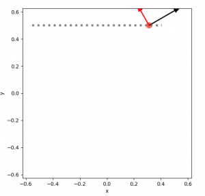
If you have only one distance vector (and the compass direction, which is assumed for all of these), it's easy to see that it's pretty unconstrained:
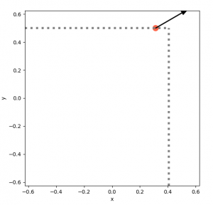
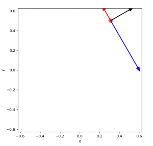
With that one vector, it could be anywhere on that dotted gray line. Adding another vector narrows it down, but you can see that it can still "slide" along the dotted line and satisfy both vectors:
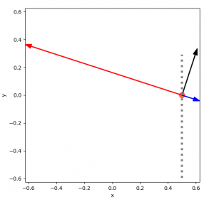
Finally, three uniquely determines its position:
This isn't too hard to figure out visually, but it actually ends up being a bit of a pain to write. For example, you can't assume that the vectors have exactly the value they should, so that messes with some constraint problem setups. You can probably pose this as a convex minimization problem, but I think you'd really actually need to set it up as a set of them, because it's a different equation depending on the angle (i.e., which walls it's able to hit). This is kind of what I ended up doing, but I wouldn't call it pretty.
Lastly, there are actually a small subset of cases where even three vectors don't solve it!
Now, I think if you were willing to put the TOFs at non-right angles to each other, for example, maybe the center one at $\theta$ and the other two at $\pm 10^\circ$, that would remove this case. But, from my experience with this, I'd rather get much different TOF readings that have this weakness than 3 ones that are nearly the same.
Anyway, whenever I talk about the position, it's the estimated position from the TOFs and compass.
The results!
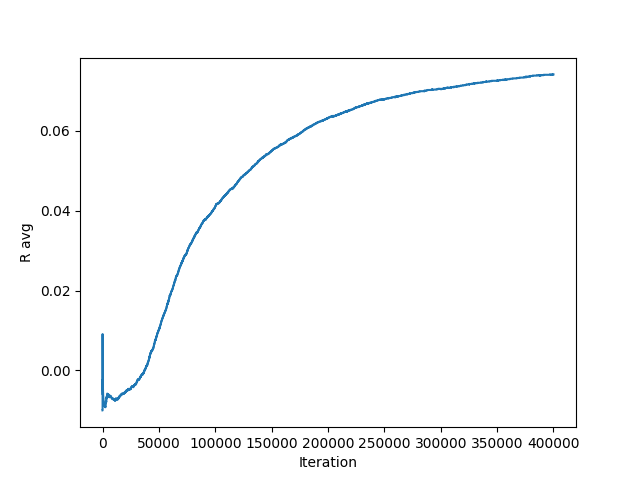
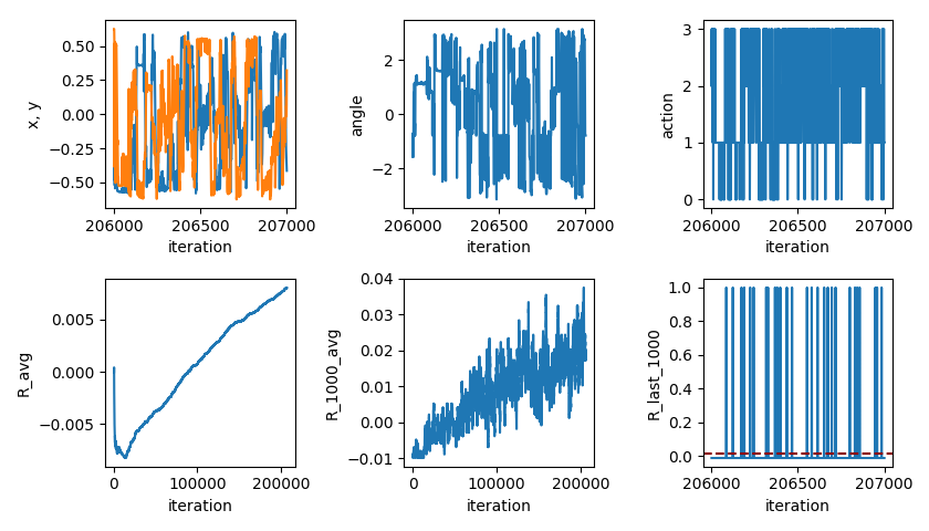
It was tricky for me to predict how long it would take to train. In the simulations above, you can see that it takes ~400k iterations to learn and level off. While this takes ~10 min or so to learn by simulating on my laptop, the robot has to, well, do it physically, which obviously takes longer. I was pleasantly surprised to find it taking a little less than 1 second an iteration, because I expected more. Even so, at 400k iterations, that would take a loooooong time. On the other hand, it's not a direct comparison with the number of iterations, because to do that, you'd really have to match the distances that the simulation/real robot go in an iteration. Anyway, let's see what happened!
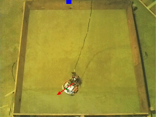
To start, here's a look at a (sped up) and labeled gif of it at the end of training!
This training took about 30 hours. The blue rectangle shows the current target. The red arrow shows the current estimated position and angle of the robot. You can see that the compass direction is almost always accurate, but the position is often somewhat off, and occasionally very off. The TOF sensors are usually pretty accurate, so the big errors in position are due to the method of calculating the position, which occasionally gets it wrong.
You can see that when it's getting the wrong position, it gets stuck in a small loop where it's choosing its next action based on where it thinks it is (it only gets out of it because there's an $\epsilon_{min}$ value of the epsilon-greedy policy). So it could eventually figure out that that "deceptive" position isn't actually accurate, and update the Q value to account for that, but that could also potentially screw it when it's in that actual position.
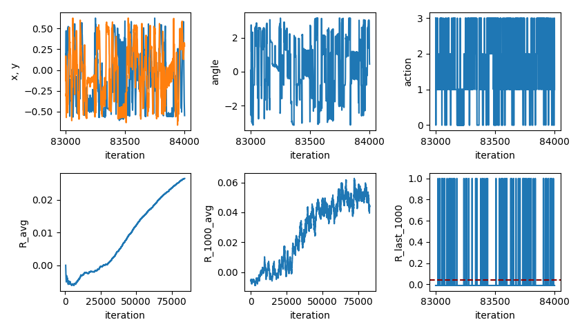
Here's what the first successful reward learning curve looks like:
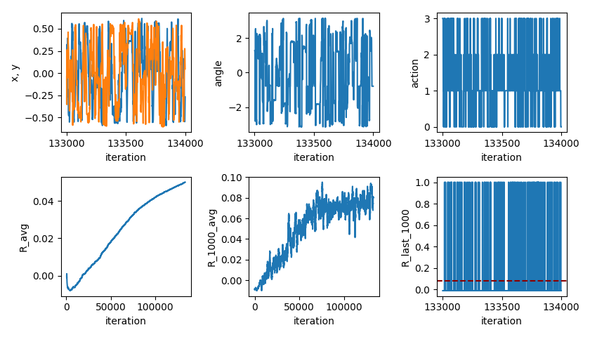
You can see that it increases pretty steadily until about 70k, at which point it levels off. I was a little surprised that it starts improving so quickly. The leveling off is where it reaches its limits (i.e., how many targets it can hit, on average, with it doing optimal actions). Actually, it might continue to improve a little... The bottom left plot is the total average reward, up to that iteration. The bottom center plot is the average reward over the last 1,000 iterations (hence why it's noisier but larger/more current).
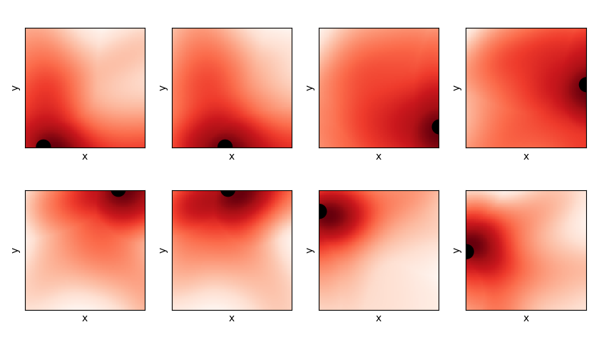
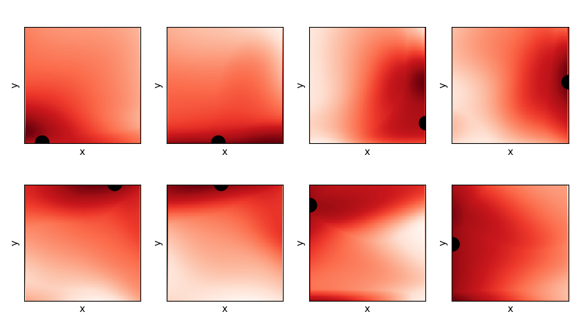
Let's also take a look at the final Q values. A state vector is of the form $(x, y, \theta, x_t, y_t)$, so to plot Q as a function of x and y, I have to specify the target and an angle. For all of the plots below, the angle is fixed at 0 degrees, and the position of the target is shown as the black disc. This gives me an output vector of the NN, which is the Q value for each of the 4 actions. To get an idea of how the Q value looks, I take the maximum of this output vector at each point, which gives the plots below (red = higher value). You can see that the maximum Q value increases as it gets closer to the target, which is expected.
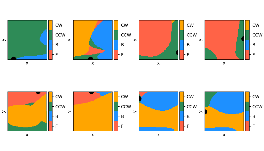
Similarly, instead of taking the maximum Q value at each point, we could look at the argmax of the output vector, which dictates which action it would take in that position. These are plotted for each target position, same as the Q plots above. Each color corresponds to the optimal action in that position (according to the robot). For clarity, these are all for $\theta = 0$, too.
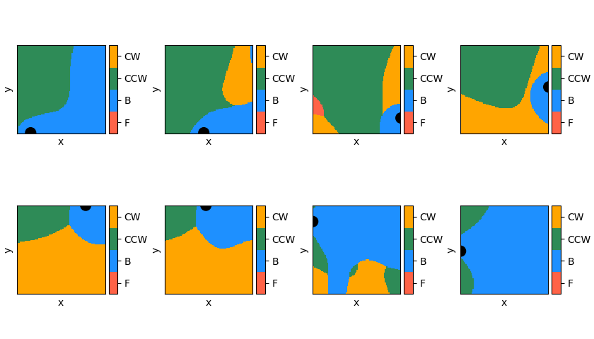
They make some sense, but to be honest, they're also a little confusing: for the 3rd and 4th ones in the top row (i.e., the targets on the right wall), it really seems like the optimal action would be to drive forward, if the target is directly to the right (because $\theta = 0$). However, apparently it wants to turn first. All I can assume is that it hasn't collected enough evidence to know that that's a superior move, so currently it is doing another set of actions, like turning, and then going to the target via some other path, that it's found to work well enough.
It's also interesting to see how the Q function and greedy action plots evolve as the robot learns. Since I saved the NN parameters after every 1000 iterations, I can do the same as above at many different points:
If you carefully compare the Q plot and the action plot, you can often actually make out regions with weird contours in the max Q value that correspond to the boundary between different actions. I suspect what's going on here is that the Q value for that action (in that position) is incorrectly too high, because it hasn't finished learning yet. Indeed, looking at the action plots, you can see that they make sense in general, but there are definitely parts that aren't the best move you could make there. This makes sense: in a given position, it can take a slightly more roundabout way to get to the target, which costs a bit of reward. After the $\epsilon$ has decayed to its minimum (0.05), if it has a suboptimal "path" that still reliably gets it to the target, it will almost always take that. Theoretically, it should eventually learn the optimal action (because $\epsilon_{min} = 0.05$), but even if it does do the slightly better move, it's only saving a little bit of time/reward, and it has to do that perhaps many times to overcome the already-established suboptimal action's Q value.
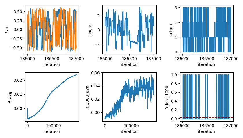
The targets were a little too sensitive at this point (getting triggered when it was too far away), so I decreased the sensitivity and trained it again, with similar results:
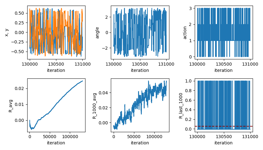
You can see that it's pretty similar, but the R levels off at a smaller number and a little later, because it doesn't get rewarded as often. This sensitivity is what I used for the rest.
Next, I wanted to try giving the NN the distances from the TOFs directly, rather than calculating the position manually. Given what a pain it was to write a function to calculate them, I was curious about how well the same simple (one hidden layer, 50 nodes) NN would do with this task...
Well... it learns, but takes ~200k iterations to do about half as well. It's not clear to me if it's starting to leveling off, but I didn't want to run it for another several days to find out. I suspect it can only do that problem so well with a single layer and that number of nodes.
So, I tried adding another layer. At first I thought that maybe the bottleneck was the single layer, so I could use two layers with fewer nodes in each (I was concerned that running pytorch on a Raspberry Pi might be too hefty for it). I tried using two hidden layers, with 20 nodes each, and found pretty terrible results. So, I tried two layers, each with the original number of nodes (50), with better results:
Much better!
I've added the distances for each TOF sensor at every point, in the direction they're aiming, to give you a rough idea of how accurate they are. You can see that they're generally pretty accurate, even at somewhat sharp angles with the wall (there's also some amount of inaccuracy with how I labeled/processed the images to make the vid).
We can also plot the Q function and best actions for this NN, though it's a little harder because the NN now takes a state vector with distances instead of the position, so for each position, I have to calculate the distances it would find (ideally) to each wall, and plug those in...
Definitely messier than the position ones, though.
However, this made me wonder: I hadn't tried the two hidden layer NN with the original method of calculating the position for it, because a single layer had worked well enough; how much better would using two layers with that be?
Apparently, it learns a little faster and does a little better, but certainly diminishing returns.
Anyway, I think that's all for now! A few random closing thoughts:
- I started this project on a whim thinking it would be dinky and easy, but it ended up actually being a huge learn. There were lots of baffling moments and pulling-out-hair debugging, but it was really satisfying to make a large system with a bunch of separate parts all work together.
- So, so much can go wrong with physical projects (not to say purely software things can't be nightmares too!). It actually felt like a real life example of "reward hacking", where I want the robot to do the goal of learning successfully, but it feels like the robot is pathologically exploring all the ways it can make something go wrong and break itself (just a vague analogy). To abuse the analogy a little more, it feels like what you see people do with reward shaping, where it's a game of trying to "plug all the leaks" until there are no more. I'll do a post in the future covering the million details I had to learn and fix.
- Along the same line, I found that long term robustness is a very different game. I've worked on tons of projects before, but I'd say the majority of them were things where you'd use it sporadically and "actively". On the other hand, this both had to run continuously for days on end, and pretty much without my supervision.
Later!